Download
1 / 155
1.6k likes | 2.01k Vues
Lecturer:. Prof. Hung-Yuan Chung, Ph.D. Department of Electrical Engineering National Central University. Text book : ‧K. J. Astrom & B. Wittenmark : Adaptive Control, second edition, Addison Wesley1995. ‧J.-J Slotine & W. Li : Applied Nolinear Control, Prentice-Hall, 1991.

E N D
Lecturer: Prof. Hung-Yuan Chung, Ph.D. Department of Electrical Engineering National Central University
Text book : ‧K. J. Astrom & B. Wittenmark : Adaptive Control, second edition, Addison Wesley1995. ‧J.-J Slotine & W. Li : Applied Nolinear Control, Prentice-Hall, 1991. ADAPTIVE CONTROL
CHAPTER 1 WHAT IS ADAPTIVE CONTROL?
Parameter adjustment Controller parameters Setpoint Controller Plant Output Control signal Figure 1.1 Block diagram of an adaptive system.
A Brief History Figure 1.2 Several advanced flight control systems were tested on the X-15 experimental aircraft.(By courtesy of Smithsonian Institution.)
Feedforward Feedback Process u y Σ -1 Figure 1.3 Block diagram of a robust high-gain system.
Judging Criticality of Process Variations EXAMPLE 1.1 Different open-loop responses Figure 1.4 (a)Open-loop unit step responses for the process in Example 1.1 with a = - 0.01 , 0 and 0.01 .(b)closed-loop step responses for the same system,with the feedback .Notice the difference in time scales.
Figure 1.5 (a) Open-loop and (b) closed-loop Bode diagrams for process in Example 1.1.
EXAMPLE 1.2 Similar open-loop responses Figure 1.6 (a) Open-loop unit step responses for the process in Example 1.2 with T= 0 , 0.015, and 0.03 .(b)closed-loop step responses for the same system,with the feedback .Notice the difference in time scales.
Figure 1.7 Bode diagrams for the process in Example 1.2. (a) The open-loop system; (b) The closed-loop system.
1.3 EFFECTS OF PROCESS VARIATIONS Nonlinear Actuators
EXAMPLE 1.4 Nonlinear valve , PI controller Valve Process u v y f(‧) -1 Figure 1.8 Block diagram of a flow control loop with a PI controller and a nonlinear valve.
Figure 1.9 Step responses for PI control of the simple flow loop in Example 1.4 at different operating levels.The parameters of the PI controller are k=0.15,Ti=1.The process characteristice are and .
Flow and Speed Variations EXAMPLE 1.5 Concentration control (1.3) Where Introduce (1.4) the process has the transfer function Figure 1.10 Schematic diagram of a concentration control system.
Figure 1.11 Change in reference value for different flows for the system in Example 1.5.(a)Output c and reference concentration,(b)control signal.
Flight Control EXAMPLE 1.6 Short-period aircraft dynamics (1.6) where Figure 1.12 Schematic diagram of the aircraft in Example 1.6.
Figure 1.13 Flight envelope of the F4-E.Fout different flight conditions are indicated.( Form Ackermann(1983),courtesy of Springer-Verlag.)
Table 1.1 Parameters of the airplane state model of Eq.(1.6) for different flight conditions (FC).
Variations in Disturbance Characteristics EXAMPLE 1.7 Ship steering Figure 1.14 Measurements and spectra of waves at diffedent conditions at Hoburgen.(a)Wind speed 3-4m/s.(b)Wind speed18-20m/s(Courtesy of SSPA Maritime Consulting AB,Sweden.)
EXAMPLE 1.8 Regulation of a quality variable in process control White noise y Figure 1.15 Block diagram of the system with disturbances used in Example 1.8.
Figure 1.16 Illustrates performance of controllers that are tuned to the disturbance characteristics.Output error when (a) ;(b)
1.4 ADAPTIVE SCHEMES Gain Scheduling Controller parameters Gain schedule Operating condition Commandsignal Control signal Controller Process Output Figure 1.17 Block diagram of a system with gain scheduling.
Model-Reference Adaptive Systems(MRAS) (1.7) Model Controller parameters Adjustment mechanism u y Controller Plant Figure 1.18 Block diagram of a model-reference adaptive system (MRAS)
Self-tuning Regulators (STR) Specification Self-tuning regulator Process parameters Controller design Estimation Controller parameters Reference Process Controller Input Output Figure 1.19 Block diagram of a self-tuning regulator (STR)
Dual Control (1.8) u y Nonlinear Control law Process Calculation of hyperstate Hyperstate Figure 1.20 Block diagram of a dual controller.
1.5 THE ADAPTIVE CONTROL PROBLEM Process Descriptions (1.9) (1.10)
x(t+1)=Φx(t)+Γu(t) y(t)=C(t)x(t) (1.11)
A Remark on Notation y(t)=G(p)u(t) qy(t)=y(t+1) y(t)=H(q)u(t)
Gain Scheduling Figure 1.21 Gain scheduling is an important ingredient in modern flight control system.(By courtest of Nawrocki Stock Photo,Inc.,Neil Hargreave.)
Controller Structures EXAMPLE 1.9 Adjustment of gains in a state feedback u=-Lx EXAMPLE 1.10 A general linear controller R(s)U(s)=S(s)Y(s)+T(s)
EXAMPLE 1.11 Adjustment of a friction compensator If v>0 If v<0
The Adaptive Control Problem • Characterize the desired behavior of the close-loop system. • Determine a suitable control law with adjustable parameters. • Find a mechanism for adjusting the parameters. • Implement the control law.
1.6 APPLICATIONS • Automatic Tuning • Gain Scheduling • Continuous Adaptation • Abuses of Adaptive Control • Industrial Products
Abuses of Adaptive Control Process dynamics Varying Constant Use a controller with varying parameters Use a controller with constant parameters Predictable variations Unpredictable variations Use an adaptive controller Use gain scheduling Figure 1.22 Procedure to decide what type of controller to use.
EXAMPLE1.12 An adaptive autopilot for ship steering EXAMPLE1.13 Novatune
1.7 CONCLUTIONS • Variations in process dynamics, • Variations in the character of the disturbances,and • Engineering efficiency and ease of use.
CHAPTER 2 REAL-TIME PARAMETER ESTIMATION 2.1 INTRODUCTION 2.2 LEAST SQUARES AND REGRESSION MODELS (2.1) (2.2)
(2.3) (2.4)
THOREM 2.1 Least-squares estimation (2.5) (2.6) Proof: (2.7) (2.8)
Remark 1. Equation (2.5) is called the normal equation. Equation (2.6) can be written as (2.9) Remark 2. The condition that the matrix is invertible is called an excitation condition. Remark 3. The least-squares criterion weights all errors ε(i) equally, and this corresponds to the assumption that all measurements have the same precision. (2.10) (2.11)