
Encoding Analog Waveforms into Digital Signals | PAM and PCM Signal Processing
E N D
Presentation Transcript
BASEBAND PULSE AND DIGITAL SIGNALING • Analog-to-digital signaling (pulse code modulation ) Binary and multilevel digitals signals • Spectra and bandwidths of digital signals • Prevention of intersymbol interference
INTRODUCTION • We will study how to encode analog waveforms into base band digital signals. Digital signal is popular because of the low cost and flexibility. • Main goals: • To study how analog waveforms can be converted to digital waveforms, Pulse Code Modulation. • To learn how to compute the spectrum for digital signals. • Examine how the filtering of pulse signals affects our ability to recover the digital information. Intersymbol interference (ISI).
PULSE AMPLITUDE MODULATION • Pulse Amplitude Modulation (PAM)is used to describe the conversion of the analog signal to a pulse-type signal in which the amplitude of the pulse denotes the analog information. • The purpose of PAM signaling is to provide another waveform that looks like pulses, yet contains the information that was present in the analog waveform. • There are two classes of PAM signals: • PAM that uses Natural Sampling (gating); • PAM that uses Instantaneous Sampling to produce a flat-top pulse.
Natural Sampling (Gating) DEFINTION: If w(t) is an analog waveform bandlimited to B hertz, the PAM signal that uses natural sampling (gating) is ws(t) =w(t)s(t)Where S(t) is a rectangular wave switching waveform andfs = 1/Ts ≥ 2B. THEOREM:The spectrum for a naturally sampled PAM signal is: • Where fs= 1/Ts,ωs = 2π fs, • the Duty Cycle of s(t) is d = τ/Ts , • W(f)= F[w(t)] is the spectrum of the original unsampled waveform, • cnrepresents the Fourier series coefficients of the switching waveform.
Natural Sampling (Gating) w(t) s(t) ws(t) =w(t)s(t)
Generating Natural Sampling • The PAM wave form with natural sampling can be generated using a CMOS circuit consisting of a clock and analog switch as shown.
Spectrum of Natural Sampling • The duty cycle of the switching waveform is d = τ/Ts = 1/3. • The sampling rate is fs = 4B.
Recovering Naturally Sampled PAM • At the receiver, the original analog waveform, w(t), can be recovered from the PAM signal, ws(t), by passing the PAM signal through a low-pass filter where the cutoff frequency is: B <fcutoff< fs -B • If the analog signal is under sampled fs < 2B, the effect of spectral overlapping is called Aliasing. This results in a recovered analog signal that is distorted compared to the original waveform. LPF Filter B <fcutoff < fs -B
Demodulation of PAM Signal • The analog waveform may be recovered from the PAM signal by using product detection,
Instantaneous Sampling (Flat-Top PAM) • This type of PAM signal consists of instantaneous samples. • w(t) is sampled at t = kTs . • The sample values w(kTs ) determine the amplitude of the flat-top rectangular pulses.
Instantaneous Sampling (Flat-Top PAM) • DEFINITION: If w(t) is an analog waveform bandlimited to B Hertz, the instantaneous sampled PAM signal is given by • Where h(t) denotes the sampling-pulse shape and, for flat-top sampling, the pulse shape is, THEOREM: The spectrum for a flat-top PAM signal is:
The spectrum of the flat-top PAM • Analog signal maybe recovered from the flat-top PAM signal by the use of a LPF. LPF Response Note that the recovered signal has some distortions due to the curvature of the H(f). Distortions can be removed by using a LPF having a response 1/H(f).
Some notes on PAM • The flat-top PAM signal could be generated by using a sample-and-hold type electronic circuit. • There is some high frequency loss in the recovered analog waveform due to filtering effect H(f)caused by the flat top pulse shape. • This can be compensated (Equalized) at the receiver by making the transfer function of the LPF to 1/H(f) • This is a very common practice called“EQUALIZATION” • The pulse width τ is called the APERTURE since τ/Ts determines the gain of the recovered analog signal • Disadvantages of PAM • PAM requires a very larger bandwidth than that of the original signal; • The noise performance of the PAM system is not satisfying.
Pulse Code Modulation • Pulse Code Modulation • Quantizing • Encoding • Analogue to Digital Conversion • Bandwidth of PCM Signals
PULSE CODE MODULATION (PCM) • DEFINITION: Pulse code modulation (PCM) is essentially analog-to-digital conversion of a special type where the information contained in the instantaneous samples of an analog signal is represented by digital words in a serial bit stream. • The advantages of PCM are: • Relatively inexpensive digital circuitry may be used extensively. • PCM signals derived from all types of analog sources may be merged with data signals and transmitted over a common high-speed digital communication system. • In long-distance digital telephone systems requiring repeaters, a clean PCM waveform can be regenerated at the output of each repeater, where the input consists of a noisy PCM waveform. • The noise performance of a digital system can be superior to that of an analog system. • The probability of error for the system output can be reduced even further by the use of appropriate coding techniques.
Sampling, Quantizing, and Encoding • The PCM signal is generated by carrying out three basic operations: • Sampling • Quantizing • Encoding • Sampling operation generates a flat-top PAM signal. • Quantizing operation approximates the analog values by using a finite number of levels. This operation is considered in 3 steps • Uniform Quantizer • Quantization Error • Quantized PAM signal output • PCM signal is obtained from the quantized PAM signal by encoding each quantized sample value into a digital word.
111 110 101 100 011 010 001 000 Digital Output Signal 111 111 001 010 011 111 011 Analog to Digital Conversion Analog Input Signal • The Analog-to-digital Converter (ADC) performs three functions: • Sampling • Makes the signal discrete in time. • If the analog input has a bandwidth of W Hz, then the minimum sample frequency such that the signal can be reconstructed without distortion. • Quantization • Makes the signal discrete in amplitude. • Round off to one of q discrete levels. • Encode • Maps the quantized values to digital words that are bits long. • If the (Nyquist) Sampling Theorem is satisfied, then only quantization introduces distortion to the system. Sample ADC Quantize Encode
Quantization • The output of a sampler is still continuous in amplitude. • Each sample can take on any value e.g. 3.752, 0.001, etc. • The number of possible values is infinite. • To transmit as a digital signal we must restrict the number of possible values. • Quantization is the process of “rounding off” a sample according to some rule. • E.g. suppose we must round to the nearest tenth, then: • 3.752 --> 3.8 0.001 --> 0
PCM TV transmission: • 5-bit resolution; • 8-bit resolution.
Dynamic Range: (-8, 8) Output sample XQ 7 5 3 1 -8 -6 8 -4 -2 2 4 6 -1 -3 -5 -7 Quantization Characteristic Uniform Quantization • Most ADC’s use uniform quantizers. • The quantization levels of a uniform quantizer are equally spaced apart. • Uniform quantizers are optimal when the input distribution is uniform. When all values within the Dynamic Range of the quantizer are equally likely. Input sample X Example: Uniform =3 bit quantizer q=8 and XQ = {1,3,5,7}
Quantization Example Analogue signal Sampling TIMING Quantization levels. Quantized to 5-levels Quantization levels Quantized 10-levels
PCM encoding example Levels are encoded using this table Table: Quantization levels with belonging code words M=8 Chart 2. Process of restoring a signal. PCM encoded signal in binary form: 101 111 110 001 010 100 111 100 011 010 101 Total of 33 bits were used to encode a signal Chart 1. Quantization and digitalization of a signal. Signal is quantized in 11 time points & 8 quantization segments.
Encoding • The output of the quantizer is one of M possible signal levels. • If we want to use a binary transmission system, then we need to map each quantized sample into an n bit binary word. • Encoding is the process of representing each quantized sample by an bit code word. • The mapping is one-to-one so there is no distortion introduced by encoding. • Some mappings are better than others. • A Gray code gives the best end-to-end performance. • The weakness of Gray codes is poor performance when the sign bit (MSB) is received in error.
Gray Codes • With gray codes adjacent samples differ only in one bit position. • Example (3 bit quantization): XQ Natural coding Gray Coding +7 111 110 +5 110 111 +3 101 101 +1 100 100 -1 011 000 -3 010 001 -5 001 011 -7 000 010 • With this gray code, a single bit error will result in an amplitude error of only 2. • Unless the MSB is in error.
Waveforms in a PCM system for M=8 M=8 (a) Quantizer Input output characteristics (b) Analog Signal, PAM Signal, Quantized PAM Signal (c) Error Signal (d) PCM Signal
Practical PCM Circuits • Three popular techniques are used to implement the analog-to-digital converter (ADC) encoding operation: • The counting or ramp, ( Maxim ICL7126 ADC) • Serial or successive approximation, (AD 570) • Parallel or flash encoders. ( CA3318) • The objective of these circuits is to generate the PCM word. • Parallel digital output obtained (from one of the above techniques) needs to be serialized before sending over a 2-wire channel • This is accomplished by parallel-to-serial converters [Serial Input-Output (SIO) chip] • UART,USRT and USART are examples for SIO’s
Bandwidth of PCM Signals • The spectrum of the PCM signal is not directly related to the spectrum of the input signal. • The bandwidth of (serial) binary PCM waveforms depends on the bit rate R and the waveform pulse shape used to represent the data. • The Bit Rate R is R=nfs Where n is the number of bits in the PCM word (M=2n) and fsis the sampling rate. • For no aliasing case (fs≥ 2B), the MINIMUM Bandwidth of PCM Bpcm(Min) is: Bpcm(Min)= R/2 = nfs//2 The Minimum Bandwidth of nfs//2 is obtained only when sin(x)/x pulse is used to generate the PCM waveform. • For PCM waveform generated by rectangular pulses, the First-null Bandwidth is: Bpcm= R = nfs
PCM Noise and Companding • Quantization Noise • Signal to Noise Ratio • PCM Telephone System • Nonuniform Quantization • Companding
Quantized Signal XQ Signal X Quantization Noise nQ Quantization Noise • The process of quantization can be interpreted as an additive noise process. • The signal to quantization noise ratio (SNR)Q=S/N is given as:
Effects of Noise on PCM • Two main effects produce the noise or distortion in the PCM output: • Quantizing noise that is caused by the M-step quantizer at the PCM transmitter. • Bit errors in the recovered PCM signal, caused by channel noise and improper filtering. • If the input analog signal is band limited and sampled fast enough so that the aliasing noise on the recovered signal is negligible, the ratio of the recovered analog peak signal power to the total average noise power is: • The ratio of the average signal power to the average noise power is • M is the number of quantized levels used in the PCM system. • Pe is the probability of bit error in the recovered binary PCM signal at the receiver DAC before it is converted back into an analog signal.
Effects of Quantizing Noise • If Pe is negligible, there are no bit errors resulting from channel noise and no ISI, the Peak SNR resulting from only quantizing error is: • The Average SNR due to quantizing errors is: • Above equations can be expresses in decibels as, Where, M = 2n α = 4.77 for peak SNR α = 0 for average SNR
DESIGN OF A PCM SIGNAL FOR TELEPHONE SYSTEMS • Assume that an analog audio voice-frequency(VF) telephone signal occupies a band from 300 to 3,400Hz. The signal is to be converted to a PCM signal for transmission over a digital telephone system. The minimum sampling frequency is 2x3.4 = 6.8 ksample/sec. • To be able to use of a low-cost low-pass antialiasing filter, the VF signal is oversampled with a sampling frequency of 8ksamples/sec. • This is the standard adopted by the Unites States telephone industry. • Assume that each sample values is represented by 8 bits; then the bit rate of the binary PCM signal is 8 • This 64-kbit/s signal is called a DS-0 signal (digital signal, type zero). • The minimum absolute bandwidth of the binary PCM signal is This B is for a sinx/x type pulse sampling
DESIGN OF A PCM SIGNAL FOR TELEPHONE SYSTEMS • If we use a rectangular pulse for sampling the first null bandwidth is given by • We require a bandwidth of 64kHz to transmit this digital voice PCM signal, whereas the bandwidth of the original analog voice signal was, at most, 4kHz. • We observe that the peak signal-to-quantizing noise power ratio is: • Note: • Coding with parity bits does NOT affect the quantizing noise, • However coding with parity bits will improve errors caused by channel or ISI, which will be included in Pe ( assumed to be 0).
Nonuniform Quantization • Many signals such as speech have a nonuniform distribution. • The amplitude is more likely to be close to zero than to be at higher levels. • Nonuniform quantizers have unequally spaced levels • The spacing can be chosen to optimize the SNR for a particular type of signal. Output sample XQ 6 4 Example: Nonuniform 3 bit quantizer 2 -8 -6 8 -4 -2 2 4 6 Input sample X -2 -4 -6
Companding • Nonuniform quantizers are difficult to make and expensive. • An alternative is to first pass the speech signal through a nonlinearity before quantizing with a uniform quantizer. • The nonlinearity causes the signal amplitude to be Compressed. • The input to the quantizer will have a more uniform distribution. • At the receiver, the signal is Expanded by an inverse to the nonlinearity. • The process of compressing and expanding is called Companding.
-Law Companding • Telephones in the U.S., Canada and Japan use -law companding: • Where = 255 and |x(t)| < 1 Output |x(t)| Input |x(t)|
y x x’ x’ Q(.) C(.) Uniform Quantizer Compressor Non Uniform quantizing • Voice signals are more likely to have amplitudes near zero than at extreme peaks. • For such signals with non-uniform amplitude distribution quantizing noise will be higher for amplitude values near zero. • A technique to increase amplitudes near zero is called Companding. Effect of non linear quantizing can be obtained by first passing the analog signal through a compressor and then through a uniform quantizer.
Example: m-law Companding x[n]=speech /song/ y[n]=C(x[n]) Companded Signal Close View of the Signal Segment ofx[n] Segment of y[n] Companded Signal
A-law and m-law Companding • These two are standard companding methods. • u-Law is used in North America and Japan • A-Law is used elsewhere to compress digital telephone signals
SNR of Compander • The output SNR is a function of input signal level for uniform quantizing. • But it is relatively insensitive for input level for a compander
SNR Performance of Compander • The output SNR is a function of input signal level for uniform quantizing. • But it is relatively insensitive for input level for a compander. • α = 4.77 - 20 Log( V/xrms) for Uniform Quantizer • V is the peak signal level and xrms is the rms value • α = 4.77 - 20log[Ln(1 + μ)]for μ-law companding • α = 4.77 - 20 log[1 + Ln A]for A-law companding
V.90 56-Kbps PCM Computer modem • The V.90 PC Modem transmits data at 56kb/s from a PC via an analog signal on a dial-up telephone line. • A μ law compander is used in quantization with a value for μof 255. • The modem clock is synchronized to the 8-ksample/ sec clock of the telephone company. • 7 bits of the 8 bit PCM are used to get a data rate of 56kb/s ( Frequencies below 300Hz are omitted to get rid of the power line noise in harmonics of 60Hz). • SNR of the line should be at least 52dB to operate on 56kbps. • If SNR is below 52dB the modem will fallback to lower speeds ( 33.3 kbps, 28.8kbps or 24kbps).