Variable Speed Pumping in Hydronic Systems
410 likes | 437 Vues
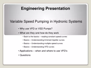
Engineering Presentation. Variable Speed Pumping in Hydronic Systems. Why use VFD or VSD Pumps? What are they and how do they work Back to the basics – reading constant speed curves Basics – Understanding trimmed impeller curves Basics – Understanding multiple speed curves

Variable Speed Pumping in Hydronic Systems
E N D
Presentation Transcript
Engineering Presentation Variable Speed Pumping in Hydronic Systems • Why use VFD or VSD Pumps? • What are they and how do they work • Back to the basics – reading constant speed curves • Basics – Understanding trimmed impeller curves • Basics – Understanding multiple speed curves • Basics – Understanding VFD curves • Applications – when and where to use VFD’s • Questions 1
It is very often a 98% efficient boiler is placed in a 20% efficient system resulting in little to no savings in energy consumption. • We suggest putting your energy toward balancing production (boilers) with consumption (Air Handling Units, fin tube radiation, etc) by providing the proper distribution (pumping and balance).
ECM technology with wire to water savings up to 80%, at very effective cost points with Variable Speed, ECM motor and system control built into the pump itself. • These pumps are the one stop solution to system efficiency, correcting the system and distribution efficiency with boiler efficiency.
Patterson Pumps has excelled in their design and efficiencies offering better design point operating efficiency; most often offering a step down in HP for identical flow and head applications resulting in higher wire to water efficiency in addition to improving the system efficiency. • We have paired Premium Efficient Pumps with Premium Efficient Motors with the Cloud line of Variable Speed Drives.
Consumption • Production • Distribution • Variable Speed Pumping • Variable Volume Pumping • Cv’s / GPM of Coil or slightly greater 1# • Coils etc / Importance of Flow Limiting • Cv =gpm/delta P square root Train
For the coldest day of the year ~2 % of the total operating period Transition period (coldest design day)
But how is the system working during the remaining 98 % of the operating period? Transition period
H Transition period Increase of the pumping head / system noises possible Unnecessary energy consumption Duty point on coldest day of the year Q H = Pumping Head HPU Q = Flowrate VPU Transition period with standard PumpsOversizing causes by worst case situation
200 gpm = 2,000,000 Btu/Hr 500 x 20 300 gpm = 2,000,000 Btu/Hr 500 x 15 400 gpm = 2,000,000 Btu/Hr 500 x 10 Checking the system Delta T can suggest the system Load Checking the Boiler Delta T vs gas consumption gives the real efficiency. System Curve vs the Pump curve.
Variable Speed Pumping in Hydronic Systems Why use VFD’s? Global Studies Carried out by the European Commission • Pumping systems account for 22% of the world’s electrical power demand • Air Compressors 18%, Fans 16%, Cooling Compressors 7%, Other equipment 37% • In some industrial plants pumps account for over 50% of the electrical load • Rotodynamic (centrifugal) pumps account for 73% of all pumps • Positive displacement (usually piston or screw types) account for 27% • Over 95% of all pumps are oversized due to multiple butt covering! • Up to 90% energy savings can be achieved using proper VFD techniques • The pump can run closer to it’s Best Efficiency Point more frequently The result of the effect of the Affinity Law is if we can operate a 125 Hp pump at half it’s speed and maintain the desired result of it’s overall function it consumes only 5 Hp!
Pumps save electrical energy by properly applying them, check the HP of 200 gpm @ 45’ vs the HP of 200 gpm @ 12’. This is really nice. Now check out the Boiler operating at 30% vs. the Boiler operating at 85 – 95% Efficient. Really Really REALLY NICE Savings.
Variable Speed Pumping Why use VFD’s? • Impeller hydraulic forces are reduced with the square of the speed change • Bearing life is proportional to the SEVENTH power of the speed change • Longer seal life • Less vibration and flow harmonics • Lower cycling (more continual flow rates) • Lower flow velocities • Better air removal • Longer glycol life • Lower friction loss • Quieter systems • No need for energy hogs • Pressure compensated by-pass valves • Wild loop unit heaters • Longer accessory life (zone valves, expansion tanks etc – soft starting)
Variable Speed Pumping Why use VFD’s? Life Cycle Costs! LCC = Cic + Cin + Ce + Co + Cm + Cs • Cic – Purchasing cost (total can be less with VFD – ie: no bypass) • Cin – Installation and commissioning cost (can be less with VFD) • Ce – Lifetime energy cost (high savings with VFD) • Co – Operation cost (labour the same) • Cm – Maintenance cost (lower with VFD) • Cs – Cost of lost production (lower with VFD – longer equipment life) Properly applied VFD equipment can produce investment paybacks less than 2 years!
Basic Heat Theory – the Facts! Is Flow Important in Hot Water Heating or Cooling? Heat always moves from high temperature to low temperature areas. Without temperature differential there is no heat movement! Remember – Heat takes the path of least resistance (least insulation) – it does not rise. Hot air rises! What is a BTU? It’s the amount of energy it takes to raise one pound of water one degree F. One Calculation to determine flow! BTU = 500 (constant) x Usgpm x ΔT Temp Diff
Heating fluid standard is 20 degree ΔT • Today with Energy Conservation this will vary. • Heating systems 20 – 40 is standard, and engineers tend to use boiler efficiency standards where higher ΔT relates to higher efficiency. • Higher ΔT relates to lower flows and lower pumping cost and lower distribution cost. • Cooling fluid standard is 10 degree ΔT • You have to watch for humidification issues. ΔT review
1,000,000 Btu/Hr 1,000,000 Btu/Hr • 100gpm x 500 x 20 • 500 x 20 = 10,000 • 500 constant for water • 50gpm x 500 x 40 • 500 x 40 = 20,000 • ΔT and outlet temperature can make anything work GPM relates to ΔT
GPM = BTU/HR 500 x ΔT 1,000 #/hr = 1,000,000 Btu/Hr 1 #/hr = 1,000 Btu/Hr 1 ton = 12000 Btu/Hr Formula’s
Heating Basics – Pump Sizing What’s the head, capacity, voltage, pipe size & type, and overall application? You need to know… FLOW – based on heat transfer (the Train) • BTU output of the boiler(s) for the primary pump(s) and loop loads for secondary pump(s) • Design temperature differential (ΔT delta T) – dependant on application, local climate etc • Calculate flow based on laws of thermodynamics (definition of a BTU) Example: 250,000 BTU/Hr = 500 (constant) x 25 USGPM x 20 deg F Calculate: Flow for 300,000 BTU/hr @ 20 deg F design differential? 30 Usgpm Calculate: Flow for 100,000 BTU.hr @ 15 deg F differential? 13.3333 USGPM Calculate: How many BTU’s will 80 USGPM transfer @ 40 deg F? 1,600,000 BTU or 1.6 MBH!
Both thermostatic valves are open only one thermostatic valve is open characteristic of circ intersecting point = new operation point system characteristic new system characteristic System Friction Loss (Head)Is it a Pump or a Circulator? Head H Ft Flow Q USGPM
What to do with excess head Typical Pumped Primary (Constant Speed Circulator) Zone Valved Secondary
What to do with excess head Constant Speed Circulator Set point of pressure bypass valve
Safety Margin When Calculating PipingOversizing caused by friction loss safety factors Curve A actual piping duty curve B actual operating point DH Curve B corrected operating point C B Power saving DP C planned piping duty curve planned operating point A Head H Flowrate Q Flow velocity v DH = Safety margin when calculating piping means ~ 30% less current consumed A Required power P Flowrate Q
Adjustment of the Pumping CapacityTrimming Impellers? Why Not? • Decreases Pump Efficiency • One Way Trip 24 50% 60% 70% 75% 20 79% 75% 16 70% H.[FT] 12 8 4 20 30 40 50 60 70 80 90 100 110 10 120 140 130 US.gpm
Q1 n1 Q2 n2 = n1 H1 2 ) ( H1 n1 H2 n2 = n2 H2 3 ) ( P1 n1 P2 n2 Q1 Q2 Changing the speed – manual multiple speed Pumping Head H Ft Adjustment of the Pumping Capacity Volume Flow Q USGPM
1,0 • n 0,9 • n 0,8 • n 0,7 • n 0,6 • n 0,5 • n 0,4 • n Changing the speed – the VFD way! 100 93 81 speed at 60 Hz Pumping Head H % 64 speed at 50 Hz 49 36 speed at approx. 40 Hz 25 Adjustment of the Pumping Capacity Volume Flow Q USGPM
2 non-regulated pump H2 3 H1 Q2 Q1 Electronic continuous speed control (Constant Pressure) • Automatic differential pressure control 1. The sensor determined the actual pumping head. (actual value) nmax 2. The electronic discerned the difference between the set value (point 1) and the actual value. (point 2) 3. The controller reduced the speed and moves the pumping head at the actual value now. (point 3) 1 Pumping Head H Ft Speed Control Volume Flow Q USGPM
Electronic continuous speed control • control modes • ∆p-c differential pressure constant • ∆p-v differential pressure variable (max head is twice min head) • ∆p-T temperature guided differential pressure control • ∆p-cv combination from differential pressure constant (second and third area of characteristic) and differential pressure variable (first area of characteristics) • Operation modes • Automatic night setback (let down function) • manual regulator • DDC (Direct Digital Control) Speed Control Strategies
max.-characteristic (non-regulated) Dpconstant Dp variable Comparison of the power consumption power draw P1W Speed Control Comparisons volume flow Q m³/h
H Saves energy, because the load-controlled pump adjusts to system changes Δpc Δpv Q Delta PC or Constant Pressure (differential) Delta PV or Pressure Variant (max head twice min) “Delta PC” vs “Delta PV” ???
∆p-c differential pressure constant • Constant Pressure Differential Across the Pump (Hset value ) • If the inlet pressure consistant (pump away from the tank) this operates like a pressure setpoint pump • Excellent in low friction loss systems (flat friction loss curves) • Independent of the number of the opened thermostatic valves Speed Control Methods
∆p-c differential pressure constant nmax Pumping Head H Ft 2 ncontrolled 3 Dp-c 1 Hset value ∆p-c Hset value-min Speed Control Method Volume Flow Q USGPM
H [m] 4 3 2 1 0 Δp-v-duty curve 0,12 m 0,5 m 0,3 m 0,03 m 2,12 m 2,5 m 2,3 m 2,03 m 2,0 m 0 1 2 3 4 Q [m3/h] 0 m3/h 2 m3/h 3 m3/h 4 m3/h 1 m3/h 2 m 2 m 2 m Δp-c-duty curve 2 m Typical Heating Pipe System with p-c Pump Control
∆p-v differential pressure variable • The maintained differential pressure-set value of the pump is changing linear between Hset value and ½ Hset value . • Used in high friction loss systems with steep friction loss curves • The required differential pressure decreases rapidly with less flow Speed Control Methods
∆p-v differential pressure variable nmax Pumping Head H Ft 2 ncontrolled 1 Hset value 3 Dp-v ½ Hset value Speed Control Methods Hset value-min Volume Flow Q USGPM
Δp-c-duty curve H [m] 4 3 2 1 0 0,5 m 1,1 m 2 m 0,1 m 3,1 m 2,5 m 4 m 2,1 m 2,0 m 0 1 2 3 4 Q [m3/h] 0 m3/h 4 m3/h 3 m3/h 2 m3/h 1 m3/h 2 m 2 m Δp-v-duty curve 2 m 2 m Typical Heating Pipe System with p-v Pump Control
Type of Boiler • Low mass boilers might not like low flows • Heat Exchangers Laminar Flows • Flow Switch Operation • Paddle type flow switches might not activate • Requires a change to control (setpoint or differential) • Pressure • Temperature • No change, not a VFD application • Three Way Valves / Temperature or Pressure? • Simplicity and Reliability of Equipment • Flow • Level VFD Pump Applications – Things to Consider
Energy Rebate Template - Custom Template A -- (Tertiary Coil/Unit Pumps) Before Retrofit The existing pump _Taco Model CC250C, 5.5, A4B2C1TL, _75_gpm @ _25_’tdh, Supply _var_F, Return _+4_F 4∆T 1.0_hp _460_Voltage, _3_Phase, Actual _3.2_ Amp Draw, Average Hours Operation_8760__ After Retrofit New WILO Stratos Model __2 x 3 – 35 __, _75gpm @ _13_’tdh Supply __var_F, Return _+9__F 9∆T _3/4_hp _230_Voltage, _1_Phase, Actual _0.5_ Amp Draw, Average Hours Operation_8760__ TWO-PHASE KILOWATT (kW) = VOLTS x AMPERES x POWER FACTOR x 2 1000 THREE-PHASE KILOWATT (kW) = VOLTS x AMPERES x POWER FACTOR x 1.73 1000 New WILO Pump 0.21kW = 0.5 x 230 x .91 x 2 0.21 x 24 x 365 x 0.07 = $129.00/year Old Taco Pump 2.32kW = 3.2 x 460 x .91 x 1.73 2.32 x 24 x 365 x 0.07 = $1,423.00/year Savings Per Year $1,294.00
Boiler Manufacturer _____________________, Model ___________________________ BTU Output ________________, Current ∆T Supply F______Return F_________ Efficiency at Current ______∆T, and ________Return Water Temperature. After WILO Stratos VFD programming to Design Conditions New Operating ∆T Supply F______Return F_______ Boiler Efficiency at Design ∆T __________________ MCF average usage at _____% Boiler Efficiency operation at lower than design ∆T and higher Return Temp. MCF proposed usage at ____% Boiler Efficiency at Design. All Boiler Manufacturers state their efficiency based upon given ∆T and inlet water temperature, each manufacturer will have many different designs so it is imperitave to get this information from them to deturmine design and current operating conditions. It is not uncommon to find most boilers designed to 20 degree ∆T for 80% efficiency operating at under 10 degree ∆T and 50% or lower efficiency. The WILO Stratos VFD controller built in can correct this deficiency with no external inputs required. This pump utilizes ECM technologies for electrical savings as well as Variable Speed control and management to improve boiler efficiencies as well as pump efficiency.
Evaporator FoulingFouling in the evaporator tubes will also increase energy costs. Fouled evaporator tubes can cause a drop in refrigerant evaporating pressure that reduces its density. As a result, the compressor must pump the gas to a higher pressure to remove an equivalent amount of heat from the chilled water. Again, the compressor must work harder, which increase energy requirements. Fouling of 0.001 Increases Energy Consumption by 10% Based on $0.07 per kWH electricity cost and Power Factor of $ 0.91 on a Efficient Chiller at 40% load = $ 0.25 kW/Ton Based on $0.07 per kWH electricity cost and Power Factor of $ 0.91 on a Efficient Chiller at 100% load = $ 0.57 kW/Ton An Example of a 500 Ton Chiller operating at 100% for 2000 hours a season, which if you averaged a seasonal load this is fairly common and fouling often exceeds 0.0042. When making ICE for thermal storage units you can modify the hours and still reach the same costs. Fouling of Reduction in Chiller Efficiency kW/Ton/100% load Wasted Energy/Ton/Season 500 Ton 0.0008 9% 0.62 $100.00 $ 50,000.00 0.0017 18% 0.672 $204.00 $102,000.00 0.0025 27% 0.724 $308.00 $154,000.00 0.0033 36% 0.775 $410.00 $205,000.00 Side stream filtration down to 100 micron filtration can save real energy dollars on chiller efficiency. ______________________ Tower Basin & Condenser Tube Cleaning Cost ______________________ Cooling Water Chemical Treatment Cost / Filtering out Solids reduces Bioside Cost by 20% ______________________ Condenser Efficiency x Tonage x kW/Ton x 2000 hours/season (Clean vs. Fouled) ______________________ Make Up Water Savings keeping TSS counts down One chiller manufacturer states without proper solids filtration efficiency is reduced by 10% in the first 24 hours of operation and continues down for the remainder of the season.