Download
1 / 120
1.2k likes | 1.36k Vues
A p* primer: logit models for social networks. Carolyn J. Anderson, Stanley Wasserman & Bradley Crouch (1999). 1. Predictive Models: Problems. Relationship specific social relation – explanatory variables

E N D
A p* primer: logit models for social networks Carolyn J. Anderson, Stanley Wasserman & Bradley Crouch (1999)
1. Predictive Models: Problems • Relationship specific social relation – explanatory variables • Response variable dichotomous/discrete (actor i does or does not have a relational tie to actor j) • The strong association between actor i’s relational tie to actor j, and actor j’s relational tie to actor i • Explanatory variables can be of several different types
2. New Family of Models: p* • Logit models & logistic regressions to Social network analysis • Models – standard response/explanatory variables • Response variable is a logit or log odds of the probability a tie is present • Explanatory variables can be general • P* easily fit approx using logistic regression software
3. Example: Friendship Data (Parker & Asher, 1993) • Study investigates the relationship between elementary school children’s friendship & peer group acceptance • Network data: children 36 classrooms (12 3rd grade, 10 4th grade & 14 5th grade) 5 public elementary schools • Total 881 children
Data collected • 3 relations (very best friendship, best friendship, friendship) • Attribute information (gender, age, race. Loneliness) • Acceptance (‘roster & rating’ how much they liked to play with each classmate)
Illustration of p* • 3 classrooms ( one from each grade) • Analyzed individually & simultaneously (differences among classes) • Fit models - emphasize dyadic effects • Reciprocity & mutuality • Ignored distinctions, created one relation reflecting friendship – either present or not
Fig. 1. The directed graph of the 5th grade classroom where the squares and circles respectively represent the boys and girls, and the arrows depict the presence of a directed friendship relational tie.
Goal • After studying each classroom individually • Want to look at similarities & differences simultaneously across the classrooms • Develop the 1stp*-type models for multiple networks
g X g Sociomatrix • Represents social relation • (i,j) entry in the matrix – value of the tie from actor i to actor j on that relation • Dichotomous Relation
Graph-theoretic Characteristics - Sociomatrix • # of ties • # of mutual dyads • Outdegree (# of relational ties) • Define actor level qualities: gender, age, grade, race, ethnicity, seniority
4. An Introduction to p* Where Ө is a vector of the r model parameters, z(x) is the vector of the r explanatory variables, and k is normalizing constant that ensures that the probabilities sum to unity. The Ө parameters are the unknown ‘regression’ coefficients and must be estimated.
The alternative version of model 2 is a logit model; not depend on k • In a logit or logistic regression model, the response variable is dichotomous and is coded as a binary variable (for example, Y *=1 or 0). • Probabilities are modeled as a function of a linear combination or a linear predictor of the explanatory variables. 4. An Introduction to p* - Logit Models
p* is a model not for the probabilities of individual ties, but for the entire collection of ties; we work with probabilities conditional on all the other relational ties in the network, not with the ‘marginal’ probabilities. • The logit version of p* by taking the logarithm of the odds; 4. An Introduction to p* - Logit p*
Fitting p* to single or multiple networks by maximizing pseudo-likelihood function • The difference in pseudo-likelihood ratio statistics can be evaluated approximately by referring the value of a distribution with degree of freedom equal to the number of parameters associated with the variable in question. • The square of such ratio is known as Wald statistics and labeled as WaldPL 4. An Introduction to p* - Fitting and evaluating logit p*
The first step in the modeling process is the identification of the effects or variables that are potentially important or interesting. • The next step is to fit simpler, more restrictive models until no simpler model can be found that does not substantially decrease the fit of model to the data. • The last step is to analyze data and interpret its results; When an estimated choice parameter is positive, the probability that a tie is present is larger than the probability that it is absent. 5. Example: a Single Class - Model Building Process
5. Example: a single class - Model Building Process e.g.) The odds that a tie is present given that two children are both girls or both boys is exp(-2.26-(-4.17))=exp(1.91)=6.75 times larger than the odds when one child is a boy and the other is a girl.
Part 6-7: p* model extension to multiple networks • Objective: to study differences among groups (different classes in Parker and Asher’s data set. For example: whether the tendencies toward mutuality are the same across networks/classes. “We need to fit all the classes in a single analysis so that we can place equality restrictions on parameters across models pp55”
6. Construct multiple networks p* model Step 1) Integrate multiple networks into one network:
6. Construct multiple networks p* model Step 2) p* model for multiple networks • Note: The explanatory statistics are not measured at the individual actor level, but are measured at graph-level. • Statistics are only meaningful at individual actor-level (non-homogeneous) is not considered here.
7. Model selection • The homogeneous effects listed in Table 4 that are likely to be important and interesting for modeling friendship relations are choice, mutuality, degree centralization, degree group prestige, transitivity, cyclicity, 2-in-stars, 2-out-stars, and 2-mixed-stars. Pp57
7. Model selection • To tease apart the effects resulting from age (or grade level) and classes requires the use of multiple classes from each grade level. • Gender is used again as a blocking factor for the homogenous effects. • Loneliness and acceptance are measured on individuals and may predict friendship ties between children. These variables can be restricted across class. Include loneliness of both sending and receiving actors. Only the acceptance ratings of the receiver are included.
7. Model selection • A tally of the number of parameters for our initial model reveals that we have 108 parameters, 36 per class: 2 for choice, 3 for mutuality, 4 for degree centralization, 4 for degree group prestige, 4 for transitivity, 4 for cyclicity, 4 for 2-in-stars, 4 for 2-out-stars, for 2-mixed-stars, 1 for acceptance ratings of the receiver, and 2 for loneliness of the sender and receiver.
7. Model selection-to simplify • Simplify the model: a. when no restrictions are placed on parameters across classes, the distributions for the individual classrooms are statistically independent. B. so we first fit the 36-prameter model for each class separately, and place restrictions within classes. C. the second round we test whether the restriction between classes is needed and whether future restrictions are possible.
8. Conclusion 1) The p* model for a single social network and the multiple network extension introduced here overcome the severely limiting assumption of independence on dyads made by earlier statistical models for such data. 2) logistic regression is easily fit to data 3) The p* model can help researchers measure study both the underlying process generating ties within single network and across multiple networks
A Practical Guide To Fitting p* Social Network Models Via Logistic Regression Bradley Crouch and Stanley Wasserman (1997) RPAD 777 Catherine Dumas
Linear Regression Review • One goal in regression analysis is to relate potentially “important” explanatory variables to the response variable of interest
Estimates of the β coefficients can be found such that the sum of the squared differences between the observed responses (Yi ) • The responses predicted by the model ( Ŷ ) is at a minimum • The least squares estimates of the regression coefficients minimize the quantity
Review Cont. • Some information about the importance of each explanatory variable from a regression by can be obtained by inspecting the sign and magnitude of the estimated regression coefficients • The model states that the response Yi changes by a factor of βj when the j th explanatory variable increases by one unit while the remaining explanatory variables are held constant
Assessing The Fit Of A Logistic Regression Model • R² is a natural measure of fit for linear regression models as it is directly related to the least squares criterion used to obtain the “best” estimates of the regression parameters • Logistic regression coefficients are estimated by maximum likelihood, using a an iteratively reweighted least squares computational procedure
The “natural” measure of model fit is given by the maximized log likelihood of the model given the observed data, and denoted by L. • We can compare the fit of two logistic regression models by inspecting the likelihood ratio statistic, where Lɍ is the log likelihood of the full model and Lʀ is the log likelihood of the reduced model (obtained by setting q of the parameters in the full model to zero)
When the full model “fits” and the number of observations is large, LR is distributed as a chi-squared random variable with q degrees of freedom
A Small Artificial Network Dataset • Fictitious network 6 organizations • Two types: Gov’t Research Organization (Circles) – Private R&D lab (Squares)
Simulation • Suppose that directional relation X= “Provides programming support to” was measured on the 6 actors involved in a software collaboration • Reason for forming collaboration – to provide equal access of programming efforts • Researcher may be interested if the organizations do provide programming support others with equal frequency
There may exist a tendency to provide programming assistance more frequently to those of their own type • One can describe the presence or absence of these tendencies in a number of ways • HOWEVER… • p* models provide a statistical framework to test hypotheses like that of “unequal access”
Presence or Absence of Certain Network Structures • If the density of ties within organizations of a certain type is greater than that outside of their type, this lends evidence to unequal access—one might call this the presence of positive differential “Choice Within Positions” • p* models postulate that the probability of an observed graph is proportional to an exponential function of a linear combination of the network statistics
The Logit p* Representation • The log linear form of p* can be reformulated as a logit model for the probability of each network tie, rather than the probability of the sociomatrix as a whole (Wasserman, Pattison) • WP defines 3 new sociomatrices:
Statistical interpretation of logistic regression models depends on the assumption that the logits are independent of one another • p*, the logits are clearly not independent • Measures such as the likelihood ratio statistic do not carry a strict statistical interpretation, but are useful as a liberal guide for evaluating model goodness-of-fit
Summary • SPSS output/Interpretation • Summary with different parameters
Recall the ‘unequal access’ hypothesis from the description of 6-actor network • It was conjectured that organizations may tend to support the programming efforts of other organizations of their own type more often than those of other types • Inspection of -2L suggests that Models 1-3 do not differ greatly with respect to overall fit, lending evidence against both the presence of differential choice within positions and a tendency for (or against) the transitivity of ties
It appears that there is no strong evidence to conclude that these fictitious organizations tend to differentially support those in either network position • It is clear that programming support is often reciprocated