Logistic Regression
Logistic Regression. Aims. When and Why do we Use Logistic Regression ? Binary Multinomial Theory Behind Logistic Regression Assessing the Model Assessing predictors Interpreting Logistic Regression. When And Why.

Logistic Regression
E N D
Presentation Transcript
Aims • When and Why do we Use Logistic Regression? • Binary • Multinomial • Theory Behind Logistic Regression • Assessing the Model • Assessing predictors • Interpreting Logistic Regression
When And Why • To predict an outcome variable that is categorical from one or more categorical or continuous predictor variables. • Used because having a categorical outcome variable violates the assumption of linearity in normal regression.
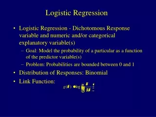
With One Predictor • Outcome • We predict the probabilityof the outcome occurring • b0 and b0 • Can be thought of in much the same way as multiple regression • Note the normal regression equation forms part of the logistic regression equation
Assessing the Model • The Log-likelihood statistic • Analogous to the residual sum of squares in multiple regression • It is an indicator of how much unexplained information there is after the model has been fitted. • Large values indicate poorly fitting statistical models.
Assessing Predictors: The Wald Statistic • Similar to t-statistic in Regression. • Tests the null hypothesis that b = 0. • Is biased when b is large. • Better to look at Likelihood-ratio statistics.
Assessing Predictors: The Odds Ratio or Exp(b) • Indicates the change in odds resulting from a unit change in the predictor. • OR > 1: Predictor , Probability of outcome occurring . • OR < 1: Predictor , Probability of outcome occurring .
Methods of Regression • Forced Entry: All variables entered simultaneously. • Hierarchical: Variables entered in blocks. • Blocks should be based on past research, or theory being tested. Good Method. • Stepwise: Variables entered on the basis of statistical criteria (i.e. relative contribution to predicting outcome). • Should be used only for exploratory analysis.
An Example • Predictors of a treatment intervention. • Participants • 113 adults with a medical problem • Outcome: • Cured (1) or not cured (0). • Predictors: • Intervention: intervention or no treatment. • Duration: the number of days before treatment that the patient had the problem.
Summary • The overall fit of the final model is shown by the −2 log-likelihood statistic. • If the significance of the chi-square statistic is less than .05, then the model is a significant fit of the data. • Check the table labelled Variables in the equation to see which variables significantly predict the outcome. • Use the odds ratio, Exp(B), for interpretation. • OR > 1, then as the predictor increases, the odds of the outcome occurring increase. • OR < 1, then as the predictor increases, the odds of the outcome occurring decrease. • The confidence interval of the OR should not cross 1! • Check the table labelled Variables not in the equation to see which variables did not significantly predict the outcome.
Multinomial logistic regression • Logistic regression to predict membership of more than two categories. • It (basically) works in the same way as binary logistic regression. • The analysis breaks the outcome variable down into a series of comparisons between two categories. • E.g., if you have three outcome categories (A, B and C), then the analysis will consist of two comparisons that you choose: • Compare everything against your first category (e.g. A vs. B and A vs. C), • Or your last category (e.g. A vs. C and B vs. C), • Or a custom category (e.g. B vs. A and B vs. C). • The important parts of the analysis and output are much the same as we have just seen for binary logistic regression
I may not be Fred Flintstone … • How successful are chat-up lines? • The chat-up lines used by 348 men and 672 women in a night-club were recorded. • Outcome: • Whether the chat-up line resulted in one of the following three events: • The person got no response or the recipient walked away, • The person obtained the recipient’s phone number, • The person left the night-club with the recipient. • Predictors: • The content of the chat-up lines were rated for: • Funniness (0 = not funny at all, 10 = the funniest thing that I have ever heard) • Sexuality (0 = no sexual content at all, 10 = very sexually direct) • Moral vales (0 = the chat-up line does not reflect good characteristics, 10 = the chat-up line is very indicative of good characteristics). • Gender of recipient
Interpretation • Good_Mate: Whether the chat-up line showed signs of good moral fibre significantly predicted whether you got a phone number or no response/walked away, b = 0.13, Wald χ2(1) = 6.02, p < .05. • Funny: Whether the chat-up line was funny did not significantly predict whether you got a phone number or no response, b = 0.14, Wald χ2(1) = 1.60, p > .05. • Gender: The gender of the person being chatted up significantly predicted whether they gave out their phone number or gave no response, b = −1.65, Wald χ2(1) = 4.27, p < .05. • Sex: The sexual content of the chat-up line significantly predicted whether you got a phone number or no response/walked away, b = 0.28, Wald χ2(1) = 9.59, p < .01. • Funny×Gender: The success of funny chat-up lines depended on whether they were delivered to a man or a woman because in interaction these variables predicted whether or not you got a phone number, b = 0.49, Wald χ2(1) = 12.37, p < .001. • Sex×Gender: The success of chat-up lines with sexual content depended on whether they were delivered to a man or a woman because in interaction these variables predicted whether or not you got a phone number, b = −0.35, Wald χ2(1) = 10.82, p < .01.
Interpretation • Good_Mate: Whether the chat-up line showed signs of good moral fibre did not significantly predict whether you went home with the date or got a slap in the face, b = 0.13, Wald χ2(1) = 2.42, p > .05. • Funny: Whether the chat-up line was funny significantly predicted whether you went home with the date or no response, b = 0.32, Wald χ2(1) = 6.46, p < .05. • Gender: The gender of the person being chatted up significantly predicted whether they went home with the person or gave no response, b = −5.63, Wald χ2(1) = 17.93, p < .001. • Sex: The sexual content of the chat-up line significantly predicted whether you went home with the date or got a slap in the face, b = 0.42, Wald χ2(1) = 11.68, p < .01. • Funny×Gender: The success of funny chat-up lines depended on whether they were delivered to a man or a woman because in interaction these variables predicted whether or not you went home with the date, b = 1.17, Wald χ2(1) = 34.63, p < .001. • Sex×Gender: The success of chat-up lines with sexual content depended on whether they were delivered to a man or a woman because in interaction these variables predicted whether or not you went home with the date, b = −0.48, Wald χ2(1) = 8.51, p < .01.

