CAVASS : Computer Assisted Visualization and Analysis Software System – Image Processing Aspects
CAVASS : Computer Assisted Visualization and Analysis Software System – Image Processing Aspects. Jayaram K. Udupa + , George J. Grevera *+ , Dewey Odhner + , Ying Zhuge + , Andre Souza + , Tad Iwanaga + , Shipra Mishra +. + Medical Image Processing Group


CAVASS : Computer Assisted Visualization and Analysis Software System – Image Processing Aspects
E N D
Presentation Transcript
CAVASS: Computer Assisted Visualization and Analysis Software System – Image Processing Aspects Jayaram K. Udupa+, George J. Grevera*+, Dewey Odhner+, Ying Zhuge+, Andre Souza+, Tad Iwanaga+, Shipra Mishra+ +Medical Image Processing Group Department of Radiology - University of Pennsylvania Philadelphia, PA *Department of Mathematics and Computer Science Saint Joseph’s University Philadelphia, PA http://www.mipg.upenn.edu/~cavass
Introduction Purpose: To present the image processing aspects of a new open-source software system called CAVASS – next incarnation of 3DVIEWNIX. (Other aspects of CAVASS are described in 6509-03, and 6519-07.) A long-standing activity in medical imaging that is begging for a definition, name, and an acronym is what we call CAVA in this presentation. CAVA: Computer-Aided Visualization and Analysis CAVA deals withthe science underlying computerized methods of image processing, analysis, and visualization to facilitate new therapeutic strategies, basic clinicalresearch,education, and training.
There is a sister activity that has come to be known as CAD: Computer-Aided Diagnosis It deals with the science underlying computerized methods for the diagnosis of diseases via images. In medical imaging, CAVA is broader in scope than CAD and predates CAD. Purpose of CAVA In:Multiple multimodality multidimensional images of an object system. Out:Qualitative/quantitative information about objects in the object system. Object system: a collection of rigid, deformable, static, or dynamic, physical or conceptual objects. CAVASS focuses on CAVA operations.
CAVA Operations Image processing: for enhancing information about and defining object system in images. Visualization:for viewing and comprehending object system in its full form, shape, and dynamics. Manipulation:for altering object system (virtual surgery). Analysis:for quantifying information about object system. CAVA operations take object system information from one space to another typically in the following sequence and also to a quantitative space.
g voxel z c a x b w u v a t r structure s pixel y scene domain b abg: body coordinate system abc: scanner coordinate system xyz: scene coordinate system uvw: structure coordinate system rst: display coordinate system
3D CAVA Software Systems brought out by MIPG DISPLAY mini computer + frame buffer 1980 DISPLAY82 mini computer + frame buffer 1982 (distributed to > 150 sites with source.) 3D83 GE CT/T 8800 1983 3D98 GE CT/T 9800 1986 3DPCPC-based 1989 3DVIEWNIX Unix, X-Windows 1993 (distributed with source to 100s of sites.) CAVASS platform independent, wxWidget 2007 CAVA User Groups UG1 – CAVA basic researchers/technology developers UG2 – CAVA application developers
UG3 – Users of CAVA methods in clinical research. UG4 – Clinical end users in patient care. Current Open Source Software Limitations LM1 – Lack of comprehensiveness of all 4 groups of CAVA operations. LM2 – Lack of coverage for user groups UG1-UG3. LM3 – Lack of adequate speed/efficiency. LM4 – Lack of adequate interfaces.
CAVASS is aimed at UG1-UG3 (not UG4 due to various legal operational, fiscal reasons) and at overcoming limitations LM1-LM4 as best as possible. Methods Key Features of CAVASS (F1) Open-source, C/C++, wxWidgets. (F2) Inherits most CAVA functions of 3DVIEWNIX. (F3) Incorporates most commonly used CAVA operations, but does not go overboard on generality and inclusiveness. (F4) Optimized implementations for efficiency.
(F5) Time intensive operations parallelized and implemented using Open MPI on a cluster of workstations (COWs). • (F6) Interfaces to popular toolkits (ITK, VTK), CAD/CAM formats, DICOM support, other popular formats. • (F7) Stereo interface for visualization. • CAVASS lays a great deal of emphasis on F3-F5. CAVA Operations in CAVASS Image Processing: VOI, Filtering, Interpolation, Segmentation, Registration, Morphological, Algebraic Visualization: Slice, Montage, Reslice, Roam through, Color overlay, MIP, GMIP, Surface rendering, Volume rendering, Animation
Manipulation: Cut, Separate, Move, Reflect, Reposition hard and fuzzy objects. Analysis: Intensity profile/statistics, Linear, Angular, Area, Volume, Architecture /shape of objects, Kinematics. The operations are listed above generically only. For each, several (popular) methods are implemented. A simplified architectural diagram of CAVASS is shown below. GUI Data Interface Graphical Interface Process Interface This paper focuses only on the image processing aspects indicated by the first of the four CAVA functions in the figure. CAVA Functions Image Proc. Vislz. Manip. Analysis
Parallelization of CAVA Operations Divide the input image into chunks and assign each chunk to a processor. A chunk represents data contained in a contiguous set of slices, either image or object structure data. CAVA operations can be divided into the following three groups. Type-1: Operation chunk-by-chunk, each chunk accessed only once. Ex: slice interpolation. Type-2: As in Type-1, but significant further operation needed to combine results. Ex: 3D rendering. Type-3: Operation chunk-by-chunk, but each chunk may have to be accessed more than once. Ex: graph traversal. CAVASS takes the following approach to parallelize Type-1 and Type-3 operations. Parallelization of Type-2 operations is described in paper 6509-03.
Parallelizing Type-1 Operations Input: Image Ii or structure(Ex: surface)Si Output: ImageIo or structureSo begin Step 1: Divide Ii or Siinto chunks. Step 2: Assign the next set of chunks to be processed to the processors, one chunk per processor. Step 3: In each processor, carry out the Type-1 operation on the chunk assigned to it and send its result to the master processor. Step 4: If there are chunks remaining to be processed, go to Step 2. Step 5: Else assembleresults from all processors and output the resulting Io or So. end
The effect of parallelization comes here from Step 3. The number of times the loop from Step 2 to Step 4 is executed depends on the size of Ii (or Si), the number of processors available, and the RAM on each processor. In this manner, load balancing is achieved automatically and there is no limit on the size of Ii (or Si) that can be handled irrespective of the number of processors available. Parallelizing Type-3 Operations Input: Image Ii or structureSi Output: ImageIo or structureSo Solutions to Type-3 CAVA operations can be characterized by optimal graph traversal algorithms. A general parallelization scheme for Type-3 operations is outlined below. It uses a queue Qj, a list Ljassociated with each chunk of the input image Ii. is a predicate whose exact form depends on the particular Type-3 operation we are dealing with.
begin Step 1: Divide Ii or Si into chunks Step 2: Initialization. A set of elements of Ii or Si are identified for initializing the underlying Type-3 operation. These are placed in the queues associated with the chunks to which they belong. Step 3: While any of the queues Qj, j=1,…,N, is not empty, do Steps 4-7. Step 4: Find a free processor Pj and load it with and Qj and Lj. Step 5: While Qj is not empty, Pjexecutes Steps 6-7. Step 6: Remove an element v from Qj, evaluate (v), and place v in Lj, perform appropriate output operations. Step 7: If (v) is true, place the appropriate neighbors of v in the queues they belong to if they are not already in their designated lists. Step 8: Combine all outputs from all processors to output Io or So. end
Parallelism is achieved via Steps 4-7. It is the task of the master processor to keep a watch on the processors whose queues become empty and who therefore may become idle. A processor may be activated becausethere are chunks whose queues are not empty. The entire process stops when all queues become empty. In Steps 6-7, the exact nature of the operations depends on the specific Type-3 operation being implemented. Step 7 also calls for inter-processor communication which can be handled in several ways to keep it efficient. The method we have implemented is to allow (slice) overlap between neighboring chunks and in the associated Qjand Lj. Multiprocessing Environment At present, there are two choices available for parallel implementation – either the multiprocessor systems (MPS) via multi-threading or via distributed processing in a cluster of workstations (COWs). After extensive experiments with several Type-1, Type-2, and Type-3 opera- tions in MPS and in a COW, we found that, COWs offer significantly
higher speed/dollar than MPS. Therefore, we report the results on a COW, except when results are compared with ITK, we used a dual processor system (3.4 GHz, 4GBRAM). Each workstation in the COW we constructed is a 3.4 GHz Pentium PC with 4GB RAM. The workstations are networked by a 1G-bit/sec connection. Results Sequential and parallel implementations of several Type-1 and Type-3 operations in CAVASS and ITK are compared using three data sets: regular, large, super. Regular:25625646 MR brain image 6 MB Large: 512512459 CT of thorax 241 MB Super: 10231023417 CT of head 873 MB (visible woman)
In the following tables, the number of processors used is shown in square brackets under “parallel”. The times reported are in seconds. No entries indicate that the operation was either not tested or not available.
The times reported in the table represent the total operational time for each listed CAVA operation. Some of these operations include a mix of Type-1 and Type-3 algorithms. We may note that pure Type-1 operations (interpolation) achieve a much higher speedup factor for parallelization than Type-3 operations (ex: fuzzy connectedness). Among the operations
listed, registration is the most time consuming. In these operations, normalized mutual information was used to register the two images. The second image was created from the first by applying a known (rigid or affine) transformation. The speedup factor achieved in this instance is excellent. With a COW of about 10 PCs, therefore, we can expect to complete a 12-parameter affine registration of extremely large data sets in about 30 minutes. Parallelized deformable registration is currently being implemented in CAVASS. Conclusions (1) COWs are more cost/speed effective than multi-processing systems. They are seemlessly expandable and upgradeable without requiring software changes.
Most CAVA operations can be accomplished in reasonable time even for extremely large data sets on COWs in portable software. • (3) COWs can be built quite inexpensively with publicly available hardware and software and standards in CAVA research labs. • (4) CAVASS can handle extremely large data sets. It seems to be considerably faster then ITK in many image processing operations. Further Information www.mipg.upenn.edu/CAVASS Release date: July/August 2007 Other papers: 6509-03 – Visualization 6519-07 – PACS