Download
1 / 30
300 likes | 401 Vues
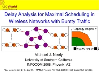
Explore the capacity region and interference sets in wireless networks for optimal scheduling strategies. Queueing dynamics and constant-factor throughput results are discussed. Sponsored by DARPA IT-MANET and NSF.

E N D
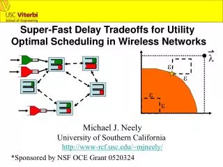
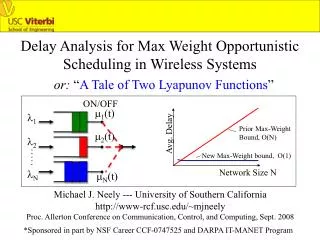
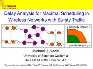
ON ON ON ON OFF OFF OFF OFF Delay Analysis for Maximal Scheduling inWireless Networks with Bursty Traffic Capacity Region L Michael J. Neely University of Southern California INFOCOM 2008, Phoenix, AZ g-scaled region gL *Sponsored in part by the DARPA IT-MANET Program, NSF OCE-0520324, NSF Career CCF-0747525
Sl = Interference Set for link lL One-Hop Network Model: N = Node set = {1, 2…, N} L = Link set = {1, 2, …, L} General Interference Set Model: Sl = l U {links that interfere with link l transmission} [Chaporkar, Kar, Sarkar Allerton 2005] [Wu, Srikant, Perkins, Trans. Mobile Comput. June 2007]
Sl = Interference Set for link lL One-Hop Network Model: N = Node set = {1, 2…, N} L = Link set = {1, 2, …, L} Example: Matching, NxN Switch Link l General Interference Set Model: Sl = l U {links that interfere with link l transmission} [Chaporkar, Kar, Sarkar Allerton 2005] [Wu, Srikant, Perkins, Trans. Mobile Comput. June 2007]
Sl = Interference Set for link lL One-Hop Network Model: N = Node set = {1, 2…, N} L = Link set = {1, 2, …, L} Example: Matching, NxN Switch Set Sl General Interference Set Model: Sl = l U {links that interfere with link l transmission} [Chaporkar, Kar, Sarkar Allerton 2005] [Wu, Srikant, Perkins, Trans. Mobile Comput. June 2007]
Sl = Interference Set for link lL One-Hop Network Model: N = Node set = {1, 2…, N} L = Link set = {1, 2, …, L} Example: Matching, Wireless Link l General Interference Set Model: Sl = l U {links that interfere with link l transmission} [Chaporkar, Kar, Sarkar Allerton 2005] [Wu, Srikant, Perkins, Trans. Mobile Comput. June 2007]
Sl = Interference Set for link lL One-Hop Network Model: N = Node set = {1, 2…, N} L = Link set = {1, 2, …, L} Example: Matching, Wireless Set Sl General Interference Set Model: Sl = l U {links that interfere with link l transmission} [Chaporkar, Kar, Sarkar Allerton 2005] [Wu, Srikant, Perkins, Trans. Mobile Comput. June 2007]
Sl = Interference Set for link lL One-Hop Network Model: N = Node set = {1, 2…, N} L = Link set = {1, 2, …, L} Example: Arb. Interference Sets General Interference Set Model: Sl = l U {links that interfere with link l transmission} [Chaporkar, Kar, Sarkar Allerton 2005] [Wu, Srikant, Perkins, Trans. Mobile Comput. June 2007]
Queueing Dynamics: -Slotted System: t = {0, 1, 2, 3, …} -One Queue for each link l: Ql(t) = # packets in currently in queue l (on slot t) Al(t) = # new packet arrivals to queue l (on slot t) ml(t) = # packets served from queue l (on slot t) Al(t) ml(t) Ql(t) Ql(t+1) = Ql(t) - ml(t) + Al(t) X(t) ={Scheduling Options} ml(t) {0, 1} ml(t) = 1 only if Ql(t)>0 AND no other active links wSl
Queueing Dynamics: -Slotted System: t = {0, 1, 2, 3, …} -One Queue for each link l: Ql(t) = # packets in currently in queue l (on slot t) Al(t) = # new packet arrivals to queue l (on slot t) ml(t) = # packets served from queue l (on slot t) Al(t) ml(t) Ql(t) Ql(t+1) = Ql(t) - ml(t) + Al(t) X(t) ={Scheduling Options} ml(t) {0, 1} ml(t) = 1 only if Ql(t)>0 AND no other active links wSl
m(t) X(t) Capacity Region: L = {All rate vectors l = (l1,…, lL) supportable} Capacity Region L [Tassiulas, Ephremides 92]: Max Weight Match (MWM) Maximize Ql(t)ml(t) Subject to: (Stabilizes Network, Supports all linterior to L)
Capacity Region: L = {All rate vectors l = (l1,…, lL) supportable} Capacity Region L Simpler “Greedy” Scheduling: Maximal Scheduling -Activate any non-empty link that does not conflict. -Keep going until we cannot activate any more links. -Non-unique solution. Easy for distributed implementation. ml(t) = 1 iif Ql(t)>0 AND no other active links wSl
Capacity Region: L = {All rate vectors l = (l1,…, lL) supportable} Capacity Region L Simpler “Greedy” Scheduling: Maximal Scheduling -Activate any non-empty link that does not conflict. -Keep going until we cannot activate any more links. -Non-unique solution. Easy for distributed implementation. ml(t) = 1 iif Ql(t)>0 AND no other active links wSl
Capacity Region: L = {All rate vectors l = (l1,…, lL) supportable} Capacity Region L Simpler “Greedy” Scheduling: Maximal Scheduling -Activate any non-empty link that does not conflict. -Keep going until we cannot activate any more links. -Non-unique solution. Easy for distributed implementation. ml(t) = 1 iif Ql(t)>0 AND no other active links wSl
Capacity Region: L = {All rate vectors l = (l1,…, lL) supportable} Capacity Region L Simpler “Greedy” Scheduling: Maximal Scheduling -Activate any non-empty link that does not conflict. -Keep going until we cannot activate any more links. -Non-unique solution. Easy for distributed implementation. ml(t) = 1 iif Ql(t)>0 AND no other active links wSl
Capacity Region L g-scaled region gL Capacity Region: L = {All rate vectors l = (l1,…, lL) supportable} Constant-Factor Throughput Results for Maximal Scheduling: [Shah 2003]: 1/2-factor, Matching on NxN Switches [Lin, Shroff 2005]: 1/2-factor, Matching on Graphs [Chaporkar, Kar, Sarkar 2005]: g-factor, General Constraint Sets [Wu, Srikant, Perkins 05, 07]: g-factor, General Constraint Sets
Prior Delay Results: Network of Size N nodes [Leonardi, Mellia, Neri, Marsan Infocom 2001]: NxN Packet Switch, full thruput, MWM, iid arrivals Delay = O(N). [Neely, Modiano, Cheng HPSR 04, TON 07]: NxN Packet Switch, full thruput, MSM-variation, iid arrivals, Delay = O(log(N)). [Deb, Shah, Shakkottai CISS 06]: NxN Packet Switch, 1/2 thruput, iid arrivals Maximal Matching, Delay = O(1).
Goals of this paper: Develop a unified treatment of throughput/delay for maximal scheduling with bursty arrivals -Develop Order-Optimal Delay Results -Treat General Interference Sets -Treat Time-Correllated “Bursty” (non-iid) Arrivals We will: Define “Reduced Throughput Region” L* Get Structural Result for General Markovian Traffic: Delay =O(log(# interferers)) 3) Tight and order-optimal (Delay = O(1)) results for 2-state Markov arrivals (such as ON/OFF processes) 4) Get Delay Bounds as a function of spatio-temporal corellations in arrival processes.
1 2 Markov Arrival Model: -Arrivals Al(t) modulated by ergodic DTMC Zl(t). -Finite State: Zl = {1, …, Ml} pl, m(a) = Pr[Al(t)=a| Zl(t)=m] for a {0, 1, 2, …} ll, m = E{Al(t)| Zl(t)=m} , ll= E{Al(t)} = ll, m pl, m m AssumeE{Al(t)| Zl(t)=m} < infinity for all states m dl Example (M = 2 states): [Possibly ON/OFF process] bl
for all lL wSl The Reduced Throughput Region L*: Capacity Region L Example: NxN Switch .7 .1 .1 .1 .1 .2 0 .3 .2 0 .3 0 .2 L* 2x2: Reduced Region L* L* 3x3: g-scaled region gL r* = 0.9 Define: L* = {(l1, …, lL)} such that: 1 lw
wSl The Reduced Throughput Region L*: Capacity Region L Example: NxN Switch .7 .1 .1 .1 .1 .2 0 .3 .2 0 .3 0 .2 L* 2x2: Reduced Region L* L* 3x3: g-scaled region gL r* = 0.9 lL 1 L*: lw L* is typically within a constant factor g of L [Chaporkar, Kar, Sarkar 05][Lin, Shroff 05] Example:(Bipartite Matching) L* is strictly larger than L/2
1 2 wSl l L Delay Analysis for Maximal Scheduling (General Interference Sets): Q(t) = Queue vector = (Q1(t), …, QL(t)) Use concept of Queue Grouping: Qw(t) QSl(t) = Lyapunov Function: L(Q(t)) = Ql(t)QSl(t) Similar Lyapunov Functions used for stability analysis in: [Dai, Prabhakar 2000] , [Wu, Srikant, Perkins 07]
E{ Ql(t) (1 - ASl(t)) } wSl wSl l L 1-step Unconditional Lyapunov Drift D(t): D(t) = E{L(Q(t+1)) - L(Q(t))} Drift Theorem: D(t) = B - B = Const Depends on Spatial Correlations E{AlAw} Aw(t) = “group” arrivals for Sl ASl(t) = Proof Uses Pair-wise Symmetry Property of the General Interference Sets: lSw iff
Quick Delay Result for Arrivals iid over slots: Suppose there is a value r* (0 < r* < 1) s.t.: r* = “relative network loading” (relative to L*) Under any maximal scheduling… Example: Simple Delay Bound for independent Bernoulli or Poisson Inputs: (independent of network size!)
Structural Delay Result for General Ergodic Markov Modulated Arrivals (finite state): Theorem: For any maximal scheduling, if r* <1 then: where |S| = 1 + Largest # interferers at any link (< N). Proof: Uses a Delayed Lyapunov Analysis technique to couple sufficiently fast to the stationary distribution. The technique is different from the T-Slot Lyapunov technique of [Georgiadis, Neely, Tassiulas NOW F&T 2006], which would yield looser (O(N)) delay results for bursty arrivals.
Structural Delay Result for General Ergodic Markov Modulated Arrivals (finite state): Theorem: For any maximal scheduling, if r* <1 then: where |S| = 1 + Largest # interferers at any link (< N). The coefficient multiplier in the numerator depends on the auto-correlation of the arrival processes Al(t): E{Al(t)Al(t+k)} (details in paper)
1 ON 2 OFF More Detailed Analysis for 2-State Markov Modulated Arrivals: dl Each Al(t) has 2-state chain Zl(t): bl Pr[Al(t) = a| Zl(t) = 1] = general dist., rate ll Pr[Al(t) = a| Zl(t) = 2] = general dist., rate ll (1) (2) Important Special Case: 2-State ON/OFF Processes: dl bl
1 2 Tight (order-optimal) Delay Analysis for 2-State Markov Modulated Arrivals: dl These Corellations are Difficult to understand! bl Challenge: Lyapunov Drift term contains: E{Ql(t)Al(t)}, E{Ql(t)Aw(t)} Solution: Use a combination of Lyapunov Drift, Steady State Markov Chain theory, and Linear Algebra. We can isolate and bound the unknown correlations!
Tight Delay Result (2-State Arrival Processes): Theorem: For any maximal scheduling, if r* <1: Where: Example: For independent ON/OFF arrival processes, we have…
ON OFF Tight Delay Result (2-State Arrival Processes): Theorem: For any maximal scheduling, if r* <1: Example: For independent ON/OFF arrival processes with 1 packet arrival when ON, we have… dl ON = 1 Packet Arrival OFF = 0 Packet Arrival bl
ON OFF Conclusions: dl ON = 1 Packet Arrival OFF = 0 Packet Arrival bl • Maximal Scheduling • General Interference Sets • Log(N) Delay Results for General Markov Arrivals • Tight and Order-Optimal (Delay = O(1)) Delay Results for 2-State Chains