Cosmology 1
Harrison B. Prosper Florida State University YSP. Cosmology 1. Topics. Island Universes The Expanding Universe The Universal Scale Factor Models of the Universe Summary. Cepheid Variables. Luminosity-Period Relation of Cepheid Variables. Henrietta Leavitt 1912. She deserved,

Cosmology 1
E N D
Presentation Transcript
Harrison B. Prosper Florida State University YSP Cosmology 1
Topics • Island Universes • The Expanding Universe • The Universal Scale Factor • Models of the Universe • Summary
Cepheid Variables Luminosity-Period Relation of Cepheid Variables Henrietta Leavitt 1912 She deserved, but did not get, a Nobel Prize
Island Universes 1924 – Edwin Hubble Using the work of Henrietta Leavitt, Hubble measured the distances to several galaxies and found that they are immense star systems very far from Earth
The Expanding Universe 1929 – Red Shift Drawing on his own observations and those of others, Edwin Hubble discovered that the red shift, z = (o- e) / e of the light from distant galaxies increases with distanceD. e= emitted wavelength o= observed wavelength
The Expanding Universe Hubble’s Law v = H0 D The Hubble Time D= vT D= (H0d) T T= 1/H0 For H0= 70 km/s / Mpc T~ 14 billion years. 1 Mpc (Mega-parsec) = 3.26 x 10⁶ light years (ly)
t1 = past λe t0 = today D(t1) a < 1 D(t0) t2 = future a = 1 D(t) = a(t) D(t0) λo D(t2) λe = a(t) λo a > 1 z = (λo - λe) / λe The Universal Scale Factor a(t) is the scale factor of the Universe t is cosmic time
t2 = future d(t2) a > 1 The Hubble Parameter H(t) is called the Hubble parameter The Hubble constant H0is simply the Hubble parameter H(t0) at the present epoch
Why Can We Assign a Cosmic Time? We have learned that your now and my now do not coincide as we move relative to each other. However, since our relative speeds are small relative to c, it is a very good approximation to take our nows to be the same. The same is true for galaxies. Their motions relative to space are << c. Consequently, we can assign each galaxy approximately the same cosmic time.
Models of the Universe General Relativity Einstein’s theory describes the evolution of spacetime. It can therefore be used to describe the evolution of the Universe The Cosmological Principle (Albert Einstein) The Universe is isotropic (looks the same in all directions) from every vantage point, at all times Such a Universe is necessarily homogeneous, that is, contains matter and energy uniformly distributed
Distribution of Galaxies APM Galaxy Survey, Steve Maddox, Will Sutherland, George Efstathiou & Jon Loveday
Models of the Universe – II TheFriedmann-Lemâitre-Robertson-WalkerMetric This describes a universe in which the proper distance, that isthe distance between two events that are simultaneous (dt = 0), changes with cosmic time, t. The proper distanceD(t) between simultaneous events in the Universe is given by where t0 is the lifetime of the Universe
D0, t0 L = c (t0 – t1) D1, t1 How Far Is Far ? t0 – t1 is the look-back time d0 = D(t0) proper distance between galaxies now d1 = D(t1) proper distance between galaxies then
Models of the Universe – III According to Newton’s laws, the total energy E of a galaxy of mass mat a distance Dis given by v D where M is the total mass enclosed within the sphere of radiusD writing gives
Models of the Universe – IV Alexander Friedmann 1888 - 1925 The Friedmann Equation We can write this differential equation as where
Models of the Universe – IV Problem 7: Using H0 = 70 km/s/Mpc, calculate the (critical) density ρ0 in kg/m3 as well as in the number of protons/m3. Calculate how much mass would be contained in a volume equal to that of the Earth. Give the answer in kg
Models of the Universe – V Since the Friedmann equation is a 1st order differential equation we can re-write it as follows where C is a constant determined by the initial conditions where
Models of the Universe – VI Georges Lemâitre 1927 Assume Ω0 = 1 a(0) = 0 Ω(a) = Ω0 / a3 and remember that a(t0) = 1 Problem 8: Using the above, and H0 = 70 km/s/Mpc, calculate the age of the Universe t0 in Gy according to the Lemâitre model
Summary • Expansion of Space In 1929, Hubble discovered the expansion of the Universe. • The Friedmann Equation This equation describes how the scale factor a(t) varies with cosmic time. Different cosmological models give different predictions for a(t)