Download
1 / 67
670 likes | 891 Vues
Requirements of ISR Experiments. Ian McCrea. A generic radar system. Radar target: . Physics. Engineering. Receiving antenna: A r. Transmitting antenna: G T. Power: P. To computer. TX. RX. A/D. Signal generator. Timing & Control. ISR spectral estimates, physical parameters.

E N D
Requirements of ISR Experiments Ian McCrea
A generic radar system Radar target: Physics Engineering Receiving antenna: Ar Transmitting antenna: GT Power: P To computer TX RX A/D Signal generator Timing & Control
ISR spectral estimates, physical parameters The essential job of an ISR experiment is to estimate the power spectral density (PSD), or autocorrelation (ACF) of IS radar returns as functions of space and time, with sufficient spatial and temporal resolution to resolve the medium properly, such that we can model and understand the physics. • Electron density Ne • Ion temperature Ti • Electron/ion temperature ratio Te/Ti • Mean ion mass mi • Ion-neutral collision frequency in The plasma dispersion relation, which governs the shape of the plasma power frequency spectrum,is a function of To extract physical parameter values, the measured ACFs are input to an inverse problem, which is then solved iteratively for [Ne Ti Te mi in] by the GUISDAP system (more about that later...)
Planning an ISR experiment: • What part/region of the ionosphere will we be looking at ? • D, E, F or the topside ? Vastly different densities, scale sizes... • Which radar system(s) will be used ? • Different operating frequencies, antenna gains, power levels.... • What time resolution are we aiming for ? • what we can achieve in practice is essentially a function of S/N • Which physical parameters do we plan to extract ? • Only densities and temperatures, or the full five parameter set ? • What error levels can we accept ? • related to the power spectral resolution that can be achieved
Typical conditions in the ionosphere When planning an experiment, you should start from some best-guess values for Ne, Ti and Te. The Table below summarises what conditions in the ionosphere above Tromsø were thought to be like in pre-EISCAT times (Bratteng and Haug, 1971). While that model is now obsolete, the numbers are not too badly off the mark – so we use them for illustrative purposes: • NOTE: The degree of ionisation is for the most part very small: • At 300-350 km (the peak of the F layer) some 3 % , • at 100 km (the E layer) normally less than 10-4 , • at 70 km (D layer), in exceptional circumstances, it can be 10-5
ISR systems parameters When planning an experiment, you also need values for all the following parameters for the ISR system you will be using: • Operating frequency / wavelength fradar / radar • TX peak power P • TX duty cycle • Max. and min. TX pulse length tmin, tmax • Max. pulse-repetition frequency PRFmax • Receiver noise temperature Tnoise • Receiver bandwidth B • Antenna gain / collecting area G, A
Figure-of-merit of ISR systems fradar , P, , Tnoise and G all influence the SNR that a radar will produce from a given plasma density at a given range, and thus indirectly the time resolution. For some examples see the Table below: tmin, tmax and B control the radar range and spectral resolution (more later)
Which parameters can we actually control ? The notion of designing experiments implies that some aspects of how the ISR system works are actually under your control. In most ISRs there are essentially only two subsystems that you can really manipulate freely – - Antenna - pointing / scanning - dwelltimes - beam selection (when multiple beams available) - Transmitter modulation - frequency - phase - coding - pulse duration
Scale heights, tidal wave modes and spatial resolution The scale height, H, of an atmospheric constituent is the height over which its density varies by 1/e. For the plasma part, this is Hp = k (Te + Ti)/ (mi g) The atmosphere also supports different vertical tidal wave modes.Ballpark lower limits for scale heights and tidal wavelengths in the auroral zone atmosphere are tabulated below: Well-designed experiments should provide height resolutions substantially better (~ 3-4x) than these values at each altitude.
Range resolution: the range-time diagram Range R = ct h0h0 =c ttx time 0 ttx t(h0)= h0/c + ttx/2 RX A sample taken at t = 2 h0/c + ttx contains contributions from the range (h0-h0/4.......h0 +h0/4), i.e. the range resolution is = c ttx/2
Altitude/range resolution and pulse length : Following the sampling theorem, select the basic pulse length, tB, such that (assuming a vertically directed antenna beam) c tB < ½ inf { - the neutral scale height, - the ionised scale height, - the shortest tidal mode wavelength } NOTE: The resulting upper bound on tB is set by the medium and must be met independently of fradar / radar !!! NOTE: In the E region, the scale height of the ionised component drops rapidly; below 100 km one often encounters very narrow Es layers with 1/e widths of just a few hundreds of meters. In the mesosphere, height resolution down to < 100 m is useful tB < 0.6 s !
Altitude resolution and modulation BW A height resolution of dR meters requires a square pulse of length t: t = 2 dR/c In the frequency domain, this pulse has a St = c(sin x/x)2 PSD, where the full width of the main lobe is Bt c / dR Examples: dR t Bt 150 m 1 s 2 MHz 1.5 km 10 s 200 kHz 15 km 100 s 20 kHz 150 km 1 ms 2 kHz
Beam (transverse) resolution The transverse (cross-beam) resolution of an ISR is defined by the antenna beam pattern.The half-power width of the main beam of an aperture antenna of size D, operating at wavelength , is approximately (we will see later why that is so). Example: For D = 32 m and = 0.33 m (EISCAT UHF), = 0.59o = /D D At a distance of R, this corresponds to a transverse resolution of rt = R Example: For R = 100 km rt = 105 . 0.33/32 = 1.03 km The beam resolution eventually becomes the limiting factor when observing in the E region with a tilted beam ( < 45o); then the beam covers about 2 km or more along the vertical direction at 100 km altitude !
Radar equation, cross sections, noise and S/N • To estimate the statistical accuracy of our experiment, we first need to establish what signal-to-noise ratio (S/N) to expect, • From the radar equation for a monostatic ISR and a beam-filling target we derive an expression for the returned signal power, • The signal bandwidth and system noise temperature determine the noise power according to Friis’ formula. But to get a value for the signal bandwidth we must first estimate the ion-acoustic frequency at each altitude, • Numerical values are inserted and actual S/N ratios computed. • We will show later that instantaneous S/N values in the order of the inverse of the number of element pulses in the modulation pattern are optimum from the statistics point of view; larger S/N is uneconomical ! • We must sometimes accept very low S/N; then we may have to average over time.
Ionospheric plasma as a radar target • Ionospheric plasma is a beam-filling radar target: • The transmitter beam is always filled with scattering electrons at some average density Ne, regardless of beamwidth and distance to the measuring volume • So the total scattering cross section,tot, is inversely proportional to transmitting antenna gain and proportional to distance squared, polarisation and average density of scatterers: • tot Gt-1 R2 sin2χ Ne
Radar equation for beam-filling targets • Power scattered from a beam-filling target of thickness dR at R = • Psc =Pt GtTot/ (4R2) = Pt Ne dR sin2χ • Power density of echo signal at radar: • dPsc/dA = PtNe dR sin2χ / (4 R2) • Power captured by receiving antenna: • Pr = ArdPsc/dA = ArPtNedR sin2χ /(4 R2) • Pr now varies only as R-2, not as R-4 as in the point target case!
Plasma radar cross section The scattering cross section per plasma electron is : = e {1 – (1 + 2)-1 + [(1 + 2) (1 + 2 + Te/Ti)]-1}, = 4 D/ where D is the plasma Debye length. For >> D and ”normal” Te/Ti ratios this reduces to: ~ e(1 + Te/Ti)-1 (0.2 ..... 0.5) e (We will return to the case of ~ D in a little while...)
Total radar cross section of a slab of F layer plasma Plasma is a beam-filling, diffuse target: Typical parameter values at 300 km altitude: h = 15 km r = 2 km ne = 3 1011 m-3 total= 5.7 10-6 m2 !!! r h ne h = slab height, defined by sampling r = slab width, defined by antenna beam ne = average electron density in slab Total cross section total : total 3/2 r2 h neT
Target, modulation and signal bandwidths The spectrum of the scattered signal, Ss, is the convolution of the modulation spectrum Sm and the target spectrum S: Ss = conv [S, Sm] whereSm St A practical approximation of the bandwidth of Ss is then: Bs = B + Bt The shape of the target spectrum, S , is defined by the plasma dispersion relation, which we will soon take a closer look at.
How SNR varies with range To get a qualitative idea of how S/N varies with range, we combine all the ionospheric factors into a ”figure of difficulty” FD(R), proportional to S/N when dR and the radar parameters are fixed: FD(R) = Ne(R) /{ R2 (1 + Te(R)/Ti(R)) fIA(R))} Figure 1 shows how FD(R) varies with altitude as a function of the ionospheric conditions, again assuming the Bratteng and Haug ionosphere and low-bandwidth modulation. We assume a radar frequency around 930 MHz and a vertical radar beam such that R=H. OBSERVATION: In an average ionosphere, FD(R) varies by over two orders of magnitude over the (100-600) km range !!
Cosmic Radio Noise An antenna pointing skywards sees a noise background of cosmic origin. At VHF and UHF, most of this is due to synchrotron radiation from free electrons orbiting in stellar and interstellar magnetic fields. Over narrow frequency ranges below ~ 1 THz, the background radiation can be fairly accurately described as blackbody radiation, whose power density (power per unit bandwidth), dPN / dB, is: dPN = kTsky dB where Tskyis the equivalent blackbody temperature or the equivalent noise temperature. Since the background radiation is beam-filling, the antenna gain does not enter into the formula. At 928 MHz (the EISCAT UHF frequency), Tskyis approximately 10 K => dPN/d = 1.38 10-22[watts/Hz]
Antenna / Receiver Noise The random thermal motion of charge carriers in lossy conductors generates noise power Ploss , which adds to the noise applied from the outside. The active devices in the receiver also add noise power, Pn , which is largely non-thermal: PantPlossPnGPPout The first generator is the antenna. The total noise power delivered by it (including cosmic noise) is Pant . The second generator is the noise generated by transmission line losses between antenna and receiver. The third generator represents the receiver noise mapped back to the input.The amplifier is assumed to be noiseless with gain GP Over the bandwidth of an IS ion line, we can treat all noise generators as blackbodies and assign equivalent noise temperatures Tant, Tloss andTn to them.
Signal-to-Noise Ratio The total (signal + noise) power per Hertz at the receiver output is: dPout/dB = dPr/dB +dPNoise/dB = GP (dPr/dB) + GP k (Tant +Tloss + Tn) = GPArPtNedR sin2χ / (Bs 4 R2) + + GP k (Tant +Tloss + Tn) So the signal-to-noise ratio (S/N) becomes S/N = ArPtNedR sin2χ / (Bs 4 R2) k (Tant+Tloss+Tn) We still need a value forBs....
Dispersion relation for ion-acoustic waves The bulk of the scattered power is contained in the ion line, which is produced by scattering off low-frequency ion-acoustic waves propagating along the scattering k-vector direction, towards or away from the radar. Ion-acoustic waves are non-dispersive, i.e. their phase velocity does not depend on their wavelength. In one dimension, theion-acoustic branch of theplasma dispersion relation looks approximately like this: (/)2 = mi-1 k (Te + Ti) = cs2 where designates the ion-acoustic wave vector andkis Boltzmann’s constant. Solving for the wave frequency: fIA = (2)-1 [mi-1 k (Te + Ti)] ½ = Λ-1[mi-1 k (Te + Ti)] ½ which shows that if we can measure the ion-acoustic spectrum, we should be able to deduce something about the temperatures...
Ion line spectral width For radar back-scatter, whereΛ= radar/2,the frequency of undamped ion-acoustic waves matching the mono-static Bragg criterionΛ= radar/2is fIA= [mi-1 k (Te + Ti)] ½• (2 f radar / c) We can use this to compute a zeroth order estimate of the spectral width of the ion line return, B: Ne = 5.0 1011 m-3 Ti = 1020 K Te = 2400 K mi = 16 amu (100 % O+) For the EISCAT UHF (930 MHz) fIA = 8.27 kHz => B 2• fIA = 16.6 kHz fIA 8.89 10 -6 * f radar
Real (Landau-damped) ion line spectra are wider by ~ 60 % : LEGEND: Red – F region (300 km) ne = 3 .1011 Te = 2000 K O+ Ti = 1000 K Green - F region (300 km) ne = 1 .1011 Te = 3000 K O+ Ti = 500 K Blue – E region (120 km) ne = 5 .1010 Te = 300 K NO+ / O2+ Ti = 300 K Black – topside (1000 km) ne = 5 .1010 Te = 4000 K 90%O+ 10% H + Ti = 3000 K Spectra computed for the EISCAT UHF radar wavelength of 0.33 m (930 MHz). Power spectral density (y-axis) plotted to linear scale
How dPr/dB varies with range Monostatic radar equation for beam-filling targets: Pr = ArPtNe dR (Te,i) / (4 R2) The target range, R, affects the received power directly: Pr R-2 The electron number densityNe is a function of R: Pr Ne(R) The effective scattering cross section is also a function of R: Pr (Te,i (R)) = e(1 + (Te (R) /Ti (R))-1 We assume that the scattered power is spread fairly uniformly across the ion line bandwidth, B,which in turn is a function of Te,i: dPr/d B-1(Te,i ) = B-1(Te,i (R)) (2 fIA (R))-1
An added complication: the Debye cutoff So far, we have assumed that = 4 D/ << 1 But at altitudes above 500 km, becomes significant and we must use the full expression for ionto estimate the S/N ratio: ion () = e [(1 + 2) (1 + 2 + Te/Ti)]-1 We note that (assuming Te/Ti = 1), ion ( = 1) = 0.33 ion ( = 0) This ”Debye cutoff” can become a problem for UHF ISR systems. Refer to Figure 2, where the 33 % - cross section heights are indicated on two typical ionosphere profiles. At 930 MHz, measurements at all heights > 500 km will suffer badly under minimum ionospheric conditions...
Now we can finally estimate S/N (h): • dRtBt Bs , dPr/dB • h, Ne, Te, Ti B, Pr • Tsky , Tloss , Tn PN S/N (h)
S/N: some numerical examples We use the parameters of the EISCAT UHF system, the Bratteng and Haug model ionosphere, a slab height dR appropriate to the scale height and sin2χ = 1 (mono-static operation) to work a couple of examples: f = 9.28 108 Hz Tsky = 10 K P = 1.3 106 W Tn = 35 K A = 560 m2 Tloss = 55 K
How Spectral Information is Derived Range R = ct h0 time 0 ttx t(h0)= h0/c + ttx/2 Point target at h0 illuminated from t = h0/c to t = h0/c + ttx 2h0/c 2h0/c + ttx RX amplitude A(t) sampled from t = 2h0/c to t = 2h0/c + ttx ; FFT or autocorrelationcomputed
How fast, and for how long, must we sample? Obviously, the receiver bandwidth BW must be > Bs to pass all spectral information on to the sampler. For low-bandwidth modulations (i.e. long pulse), Bs B and we can argue as follows: How fast: The sampling theorem tells us that fsamp > 2 * fmaxsamp < (2 * fmax )-1 where fmax is the highest ”nonzero-power” frequency in the signal spectrum (e.g. ~ 50 kHz in the 300-km model spectrum) For how long: Depends on which, and how many, parameters we want to get out from the subsequent analysis ! This is best illustrated in the time domain...
The plasma autocorrelation function, rxx() is the Fourier transform of the ion line power spectral density. Using the plasma dispersion relation, we can compute model autocorrelation functions for different combinations of Ne, Teand Ti(Figure 3). An estimate of the targetrxxat lag timen0can be computed from the time series of complex amplitude samples,s(t),output from the receiver: rxx(n0) = s (t) s*(t + n0) Intuitively, it may appear natural to continue sampling at a given range for so long that the model ACF has decayed almost to zero. To see if that helps at all, let us first look at how the different plasma parameters influence the model ACF at different lag times :
Partial derivatives of the plasma dispersion function: • rxx() / Ne • rxx() / Ti • rxx() / (Te/Ti) • rxx() / mi • rxx() / in are shown in terms of/0, where0, the plasma correlation time, is the time to the first zero crossing of the ACF of a undamped ion-acoustic wave with wavelength =Λ= ½ radar NOTE: rxx() / Ti and rxx() / miare almost linearly dependent...
ACF estimate extent and errors The next figure (from Vallinkoski 1989) shows how the errors of the different plasma parameters behave as functions of lag extent when measurement data are fitted to a five-parameter plasma model. Comparing this to the previous figure , we see that as the lag extent is increased to the point where the partial derivative of a given parameter goes through a complete cycle, the error in that parameter suddenly drops dramatically. If one is satisfied with slightly less than ultimate accuracy, extending the measurement to /0 = 2.5 should be sufficient. By about /0 = 3.5, all errors have settled down to their asymptotic value – But to allow for surprises, design for /0 4 !
ACF estimate, practical consequences • /0 4is actually rather long, even at 930 MHz: • 280 s at 150 km • 650 s at 100 km • Several milliseconds at 95 km • The required duration of illumination increases as the inverse of the radar frequency(~ 2700 s @ 150 km/224 MHz) • Experiments should be designed to illuminate the plasma with RF for at least this long (longerthe lower you go) ! • At the same time, the illumination must provide altitude resolution better than the smallest of (scale height, shortest tidal mode) at each altitude (and those get shorter the lower you go, see Table) ! At some point we run into a conflict...
Pulse length giving resolution equal to the scale-height. ionospheric correlation time, τ1 for UHF Time of flight for radar pulse ionospheric correlation time, τ1 for VHF Possible values for UHF experiment Minimum pulse length obtainable from transmitter Constraining factors for an incoherent scatter radar experiment Some constraining factors for incoherent scatter experiments, shown as functions of height for typical ionospheric conditions.
Summing up the various timing restrictions in one diagram : Required ACF extents at different radar frequencies progress from upper left to lower right, Pulse length limitations go from lower left to upper right. Four different regions can be distinguished: • Region I: Height resolution provided by long uncoded pulses OK, intra-pulse ACF measurement OK, • Region II: Coding required to get the desired height resolution, intra-pulse ACF measurement OK, • Region III: Pulse-to-pulse ACF measurement required. Coding not mandatory, but advantageous, • Region IV: Pulse lengths in this region do not meet the minimum ACF length requirement - BEWARE!
Pulse length giving resolution equal to the scale-height. ionospheric correlation time, τ1 for UHF Time of flight for radar pulse ionospheric correlation time, τ1 for VHF Possible values for UHF experiment Minimum pulse length obtainable from transmitter Constraining factors for an incoherent scatter radar experiment Some constraining factors for incoherent scatter experiments, shown as functions of height for typical ionospheric conditions.
Pulse-to-pulse measurements Whenever 2R/c < 40(R) it is impossible to do a full spectrum estimate of the target at R within the timespan of a single radar pulse (Region III). Instead, we can illuminate the target repeatedly with a series of pulses transmitted at some repetition frequency PRFptp and form estimates of the target ACF by taking cross-products between samples from the same height taken in different interpulse periods: rxx(r, ktptp) = s(r,np=i) s*(r,np=i+k) where tptp = 1/ PRFptp NOTE: For this to work, the radar must be pulse-to-pulse phase coherent !
Statistical accuracy and averaging The normalised variance of an individual ACF lag estimate has the general form: [var (rxx()) / rxx2()] = (k1 nind)-1 (np + (S/N) -1)2 where k1 is determined by the code and computation scheme used, np is the number of elements in the code and nind is the number of statistically independent estimates averaged: WhenS/N np-1, both terms contribute equally to var (rxx()) whenS/N > np-1, its contribution to var (rxx()) tapers off, whenS/N >> np-1, no further improvement in var (rxx()) !
The high SNR case When S/N >> 1 [var (rxx()) / rxx2()] (k1 nind)-1 np2 and the only way to reduce the variance further is to increase nind However: Measurements repeated closer in time than~ 40are partially correlated; thus we can obtain at most nind= 1/ 40 totally independent estimates per unit time ! There are two ways to work around this restriction: 1) Use as high a radar frequency as possible (as this lowers0), 2) Transmit on multiple frequencies simultaneously
PRF, max. range and rate of statistics Since [var (rxx()) / rxx2()] nind-1 it is smart to increase nind by using the highest PRF the radar can deliver. However, since max range Rmax and max useable PRF are related through PRFmax = c/ (2 Rmax) we cannot increase the PRF arbitrarily; there is a ceiling on the rate at which we can reduce variance by averaging: Rmax 150 300 1500 km PRFmax 1000 500 100 Hz Error in 1 s 3.2 4.5 10 % (asymptotic)
Range ambiguities and frequency hopping When a modulation pattern is being repeated on a given frequency with a PRF > 50 Hz or so, two or more RF packets will be in the dense part of the ionosphere simultaneously, separated in range by Ramb = c/(2 PRF) The more distant pulses will be at the so-called ambiguous ranges (1st, 2nd ). Returns from all illuminated ranges will be received simultaneously; there is no way to prevent the ambiguous-range pulses from at least producing clutter – But when the radar hardware allows it (as e.g.in EISCAT/ESR), four or more frequencies can be used in round-robin fashion, pushing the first ambiguous range out to well past 3000 km. Ambiguous returns from such ranges are normally so weak as to be negligible. CAUTION:This obviously does not work in pulse-to-pulse experiments...
Blind ranges and staggered PRF All pulsed radars have a blind range problem: You cannot receive while you transmit, The distant range being illuminated by the previous pulse during the transmission time is not observable, The fraction of the theoretically observable range that is being blanked in this way is directly proportional to the duty cycle. Difficult problem at the ESR (max = 25%), and in P-T-P work Workaround: - change PRF at intervals, or use multiple, interlaced PRFs Eliminates the total blindness, but the blind ranges will be sampled at a lower rate than the rest.... Always wastes some fraction of the available .