Spherically symmetric space-times in loop quantum gravity
230 likes | 439 Vues
Spherically symmetric space-times in loop quantum gravity. Jorge Pullin Horace Hearne Institute for Theoretical Physics Louisiana State University. With Rodolfo Gambini, Miguel Campiglia University of the Republic of Uruguay. Plan. Introduction Spherically symmetric gravity

Spherically symmetric space-times in loop quantum gravity
E N D
Presentation Transcript
Spherically symmetric space-timesin loop quantum gravity Jorge Pullin Horace Hearne Institute for Theoretical Physics Louisiana State University With Rodolfo Gambini, Miguel Campiglia University of the Republic of Uruguay
Plan • Introduction • Spherically symmetric gravity • Loop representation for spherical symmetry exterior. • Dirac quantization. • The interior problem. • Expectations for more general models.
Introduction: Spherically symmetric space-times include Schwarzschild and therefore the singularity. They are the “next obvious thing” to try with loop quantum gravity after homogeneousspace-times. Work in progress, we do not have results for the complete space-time. Models always involve a tradeoff: using special features simplifies treatment butlessens the value as lessons for the full theory. We will carry out a Dirac quantization in the loop representation and discuss implications for other approaches.
Spherically symmetric canonical quantum gravity: Previous work on the spherical symmetry with the traditional variables for canonical gravity: Berger, Chitre, Moncrief, Nutku (1973), Lund (1973), Unruh (1976), and the definitive work (in vacuum): Kuchar (1994). Kuchar does not simply use symmetry-reduced variables and proceed to a Dirac quantization, but makes a careful choice of canonical variables such that the quantization is immediate and the only dynamical variable is the mass. In thissense it can be seen as a “microsuperspace quantization”. Such a quantization has so little in common with the full theory that we cannot learnanything about, for instance, the use of loop quantization or singularity elimination. We would like to use less information about the model in question, i.e. just imposespherical symmetry and then proceed with the usual quantization program.
Suppose one considers the usual spherical (spatial) metric, And a appropriately spherical conjugate momenta. One will be left with one diffeomorphism constraint Cr and a Hamiltonian constraint H. They will satisfythe usual constraint algebra, Midi-superspaces: things complicate Remarkably, even this simple model has “the problem of dynamics” of canonical quantum gravity. This problem is absent in homogeneous cosmologies.
Previous work with the new variables, Bengtsson (1988) Kastrup and Thiemann (1993) and Bojowald and Swiderski (2005, 2006). Choose connections and triads adapted to spherical symmetry, L’s are generators of su(2). It simplifies the constraints if one introduces a “polar” canonical transformation inthe variables A, P,b,Pb To fix asymptotic problems (Bojowald, Swiderski), one does a further canonical change, Spherical symmetry with the new variables
Finally, one is left with the following form for the constraints, To simplify matters further, we will fix the spatial coordinate gauge. This eliminates the diffeomorphism constraint, but still leaves a Gauss law anda Hamiltonian constraint with a first class algebra of constraints with structurefunctions, therefore still a challenging problem. The choice is Ex=(x+a)2, which in turn puts the horizon at x=0. The variable a is a dynamical variable that is related to the mass of the space-time a=M/2. One solves D=0 for Ax and substituting in H one has an equation for thepair A,E.
And the constraint algebra is, So the model, although simplified, is still quite challenging (has structure functionsin the constraint algebra). So in principle we cannot treat it with traditional techniques, we could use the “uniform discretizations” or the “master constraint” treatment. The Hamiltonian constraint becomes, But it turns out that for this example one can introduce a trick that allows forthe traditional treatment. Dividing the constraint by E turns the Hamiltonian constraint Abelian! If one wishes to discretize things to regularize expressions, one can do it in such a way that the constraints remains first class upon discretization. Then one can quantize the discrete theory in the traditional way. But first let us construct a suitable loop representation for these models.
Manifold is a line. “Graph” is a set of edges, . The only variable that behavesas a connnection on the line is Ax. The variables h and A are scalars, so in the looprepresentation one uses “point holonomies” to represent them. Volume of an interval I Loop representation for the spherically symmetric case: To avoid presenting too many equations, I will write the states for the “gauge fixed” case we introduced. There the only variables in the bulk are E and 2gK=A We will see that thisformula has unexpected implications.
“Transverse point holonomies” and triads are well defined operators, And one can do the “Thiemann trick” (calculation omitted) for the non-polynomialportion of the Hamiltonian constraint (as in the full theory and LQC), and thatthe inverse of the triad is a bounded operator,
It turns out that it is relatively easy to solve the constraint in the connection representation. One rewrites it as, And imposing it as a quantum operator leads to states, And f is an explicit function ofelliptic integrals. With this one can represent the Abelian Hamiltonian constraint in the loop representation.We start from a classical discretization that is written in terms of quantities that are easy to promote to operators in the loop representation (i.e. replace connectionsby “small holonomies”, etc)
The bottom line is that one recovers the same quantization as Kuchař, one hasa wave function that depends on the mass C(a,t), and imposing the constraint onthe boundary one gets, How does the constraint look like in the loop representation? Start from classicallyrewriting the constraints as Om =1. Then the quantum version of O is, So one is left with only a function of the mass C0(a) as the wavefunction of thetheory, with no dynamics.
The above recursion relation can be explicitly solved and one can show thatthe solution is the “loop transform” of the solution we found in the connectionrepresentation, r identifies super-selection sector. This can be immediately represented in the loop representation as, Notice the parallels with the expression that arises the Loop Quantum Cosmology case. This is suggestive, since it might imply a similar resolution for the Schwarzschildsingularity as one had for the cosmological one. However, detailed calculations in horizon penetrating coordinates would be needed to confirm this.
Use of uniform discretizations: What if we had not made use of the trick of Abelianizing the constraints? Thenthe only approach we know is to use the “uniform discretizations”. Briefly recalling, the uniform discretizations are defined by the following canonical transformation between instants n and n+1, Where A is any dynamical variable and H is a “Hamiltonian”. It is constructedas a function of the constraints of the continuum theory. An example could be, (More generally, any positive definite function of the constraints that vanisheswhen the constraints vanish and has non-vanishing second derivatives at theorigin would do) Notice also that parallels arise with the “master constraint program”. These discretizations have desirable properties. For instance H is automaticallya constant of the motion. So if we choose initial data such that H<e, suchstatement would be preserved upon evolution.
The main challenge is to implement H as a quantum operator and checking that zerois in the spectrum. One can make use of the ambiguity of discretization to either have zero in the spectrum or to minimize the eigenvalue of the fundamental state. We use this as criterion for choosing the best discretization possible. In this model the best discretization would be the Abelian one we presented. Onecould then construct H and show that zero is an eigenvalue. Since the methodcoincides with the Dirac method for Abelian constraints, there is no need to do this. In order to illustrate what is expected to happen in more general models where onecannot find a vanishing eigenvalue for H, one can construct H for a different discretization and evaluate its expectation value on the eigenstates for the Abelianmodel. One generically gets, The operator therefore does not have a quantum continuum limit, e->0, lPlanck finite. On the other hand it does have a classical continuum limit, e->0, lPlanck->0.
Solving the eigenvalue problem becomes a (hard) problem in quantum mechanics, akin to those in solid state physics. It is encouraging that there exist establishedmethods to deal with these problems. Although an obvious over-kill for the vacuum problem, the complexity of the situationchanges little if one couples gravity to matter. One could envisage in the near future solving the “quantum Choptuik problem” of the gravitational collapse of a scalar field or the CGHS black hole using variational Monte Carlo.
The interior problem: The interior of Schwarzschild is isometric to a Kantowski-Sachs universe. Theansatz for the three geometry we considered is general enough to include thismetric, so we can also use it for the interior. The Gauss and diffeomorphismconstraints read as before, We now rewrite things in terms of gauge invariant combinations of variables Kf andKx=(Ax+h’)/g that guarantee that Gauss’ law is satisfied. The diffeo and Hamiltonian constraint take the form, And are first class. We now fix a gauge (Ex)’=0, which in turn determines thelapse N’=0. One is left with a super-Hamiltonian,
And the diffeomorphism constraint becomes which implies that K isindependent of r and is determined by the ODE, together with the form of N thatpreserves that (Ex)’=0, with solution The usual form of the Kantowski-Sachs metric arises with the additional gauge condition which implies the shift is a function of t only yielding an ODEfor the triad with solution,
Starting from a rescaled version of the the Hamiltonian constraint we had, We proceed to “holonomize” it (it is slightly easier to implement its square), Quantizing, one would have have, for a symmetric factor ordering, And one can try a solution of the form Assuming one is led to a solution scheme in powers ofPlanck’s length.
To zeroth order, To first order The zeroth order is (the product) of quasilinear equations for S. The firstorder is a quasilinear equation for C0. Similar equations arise for the Ci’s at higherorders. One can solve exactly for S, This technique can be used to provide a zeroth order approximation for the variational Monte Carlo techniques we mentioned.
It is interesting to study the classical solutions of the action we obtained.One can see that indeed they are singularity free, but they require careful tuning of boundary conditions for the tunneling through the singularity to besymmetric. V V t t This requires further study, but it might be a sign of the instabilities that have been observed in the recursion relations that appear in the loop quantizationby Cartin, Khanna, Bojowald, etc. It would be interesting to connect this quantization with the more traditional loop approach, Ashtekar & Bojowald, Modesto, etc.
As in LQC, one expects the value of the parameter of the “transverse point holonomy”, r, to take a finite minimum value, One last intriguing observation: holography?! If one acts with this holonomy on a spin network state, one adds an elementof volume, Ng, Lloyd, etc Therefore for any model based on this kinematical structure, the volume growsin discrete increments that take as minimum value the element of volume mentioned. This statement is independent of the details of the dynamics of themodel considered (e.g. it would survive coupling the theory to a scalar field, forinstance). If one considers the volume of a shell of width Dx asymptotically one has Nelements of volume per shell, Notice that it makes sense that one obtains the (spatial) Bekenstein bound in spherical symmetry, since it is known not to hold if one is in a more general situation.
Summary: • One can study spherically symmetric space-times using loop quantum gravity. • One needs to use special features of spherical symmetry to apply the traditional Dirac quantization technique. • The setup is ready, we need to extend it to horizon penetrating coordinates to make better statements about the singularity. • Without using special tricks the problem is hard, and it offers a promising arena to test new ideas for handling the problem of dynamics in canonical quantum gravity, like the “uniform discretization” or the “master constraint” approaches. • Holography and the Bekenstein bound can be connectedwith the basic elements of loop quantum gravity, irrespective of the details of the dynamics.