Software Correctness Proofs
Software Correctness Proofs. CIS 376 Bruce R. Maxim UM-Dearborn. Formal Analysis. Refers to tool-based methods used to explore, debug, and verify formal specifications Methods Theorem proving Proof checking Model checking Animation and simulation. Formal Proof - part 1.

Software Correctness Proofs
E N D
Presentation Transcript
Software Correctness Proofs CIS 376 Bruce R. Maxim UM-Dearborn
Formal Analysis • Refers to tool-based methods used to explore, debug, and verify formal specifications • Methods • Theorem proving • Proof checking • Model checking • Animation and simulation
Formal Proof - part 1 • Use deductive reasoning • Proofs are based on a formal system that includes • set of primitives • finite strings from a fixed alphabet • set of axioms • specifying the rules of behavior for the primitives • set of inference rules • allow deduction of additional true statements (known a theorems) within the system
Formal Proof - part 2 • Deductive system • axioms and inference rules for a formal system • Theory • axioms and derived theorems in a formal system • Proof of theorem • sequence of statement transformations that adheres to the system’s inference rules • s1, s2, s3, … , sn |- T • theorem T is provable following the sequence si
Formal System Properties • Consistent • not possible to derive a statement and its contradiction form the same set of initial statements • Complete • every true statement is provable • Decidable • there is an algorithm for determining whether any legal statement is true • Note: consistency must be present, completeness and decidability would be nice
Proof Construction • Forward argument (deductive calculus) • starting with axioms and proven results the inference rules are used to prove the desired consequent • Backward argument (test calculus) • starting with the desired result and applying the inference rules to derive a known result, axiom, or theorem
Program Verification • Similar to writing a mathematical proof • You must present a valid argument that is believable to the reader • The argument must demonstrate using evidence that the algorithm is correct • Algorithm is correct if code correctly transforms initial state to final state
State of Computation • Most programming algorithms are based on the notion of transforming the inputs to outputs • The state of computation may be defined by examining the contents of key variables before and after the execution of each statement
Assertions • Assertions are facts about the state of the program variables • It is wasteful to spend your time looking at variables that are not effected by a particular statement • Default assertion • any variable not mentioned in the assertion for a statement do not affect the state of computation
Use of Assertions • Pre-condition • assertion describing the state of computation before statement is executed • Post condition • assertion describing the state of computation after a statement is executed • Careful use of assertions as program comments can help control side effects
Code Verification Example • Let’s assume we have an array with a search operation that corresponds to the English specifications below • The procedure searches and array A of length N for a value X • If X is found than the value of Y is set to the array index where X was found on exit • If no array element in A matches X then Y will be set to zero on exit
Example - Formal Specifications • Pre-condition • N > 0 • Post condition • {X = A[Y] and (1 <= Y <= N)} or • {(Y = 0) and (k : (1 <= k <= N) A[k] <> X)} • Proof would need to show that algorithm transformed state of computation from pre-condition to the post condition
Simple Algorithm • Model {P} A {Q} • P = pre-condition • A = Algorithm • Q = post condition • Sum algorithm {pre: x = x0 and y = y0} z = x + y {post: z = x0 + y0}
Sequence Algorithm • Model if {P} A1 {Q1} and {Q1} A2 {Q} then {P} A1 ; A2 {Q} is true • Swap algorithm {pre: x = x0 and y = y0} temp = x x = y y = temp {post: temp = x0 and x = y0 and y = x0}
Intermediate Assertions • Swap algorithm {pre: x = x0 and y = y0} temp = x {temp = x0 and x = x0 and y = y0} x = y {temp = x0 and x = y0 and y = y0} y = temp {post: temp = x0 and x = y0 and y = x0}
Conditional Statements • Absolute value {pre: x = x0} if x < 0 then y = - x else y = x {post: y = | x0 |}
Intermediate Assertions if x < 0 then {x = x0 and x0< 0} y = - x {y = | x0 |} else {x = x0 and x0>= 0} y = x {y = | x0 |}
Understanding the While Loop • Every well designed while loop must • make progress to ensure eventual termination • must maintain the loop invariant to ensure that it is valid at each loop exit point //invariant holds here while (condition) do //invariant holds here make_progress restore_invariant //invariant and not(condition) hold here
Loop Invariant • Type of assertion that describes the variables which remain unchanged during the execution of a loop • In general the stopping condition should remain unchanged during the execution of the loop • Some people show the loop invariant as a statement which becomes false when loop execution is complete
Loop Invariant Example k = 0; //invariant: A[1], … , A[k] equal 0 //assert: N >= 0 while k < N do k = k +1; //make progress A[k] = 0; //restore invariant //assert: A[1], … , A[k] equal 0 and k >= N Note: say k=N will require an induction argument
While Loop Example • Algorithm while y <> 0 do z = z + x y = y – 1 ans = z • What does it do?
While Loop Assertions {pre: x = x0 and z = z0 and y = y0 and y0 >= 0} while y <> 0 do begin {0 < n <= y0 and z’ = z0 + n * x0} z = z + x y = y – 1 end {y = 0 and z’ = z0 + y0 * x0} ans = z {post: ans = z0 + y0 * x0}
Proof -1 • If y = 0 loop does not execute and no variables change so z = z + 0 * x = ans • If we assume that for n = k if program begins loop with y = k it will exit with ans = z + k * x
Proof - 2 • We must prove that when program begins loop with y = k + 1 it will exit loop with ans = z + (k + 1) * x • Suppose y = k + 1 at top of loop and the body of the loop executes one time x = x ‘ = x y = y’ = (k + 1) – 1 = k z = z’ = z + x
Proof - 3 • Since we are at the top of the loop with y = k, we can use our induction hypothesis to get ans = z’ + k * x’ • Substituting we get ans = (z + x) + k * x = z + (x + k * x) = z + (1 + k) * x = z + (k + 1) * x
Second While Loop Example Prod = 0 I = 0 {X and N are initialized and Prod = I * X and I <= N} while (I < N) do begin {Prod = I * X and I < N} Prod = Prod + X {Prod = (I + 1) * X and I < N} I = I + 1 {Prod = I * X and I <= N} end {loop exited with Prod = I * X and I >= N} {Prod = N * X}
Proof - 1 • Check I = 0 Verify that invariant is true Prod = 0 Prod = 0 * X = 0 If N = 0 condition is false and loop terminates If N > 0 condition is true and loop execution continues
Proof - 2 • Assume correctness of the invariant at the top of the loop when I = K Prod = K * X If K < N condition is true and the loop execution continues If K = N condition is false and loop terminates So post condition is true • So we are assuming that X0 + X0 + X0 + … + X0 + X0 = K * X0 = Prod k times
Proof - 3 • If we are at the top of the loop and execution continues the body adds X0 to both sides • Using our induction hypothesis we get (X0 + X0 + X0 + … + X0 + X0) + X0 = K * X0 + X0 k times • Which gives us X0 + X0 + X0 + … + X0 + X0 + X0 = K * X0 + X0 k + 1 times • Which can be written as X0 + X0 + X0 + … + X0 + X0 + X0 = (K + 1) *X0 = Prod
Proof - 4 • Since assuming the invariant is true for K we showed that it held for K + 1 • If the loop condition is true execution continues • otherwise is halts with I = N + 1 Prod = X0 * N
Counting Loop Example • This loop stores the sum of the first I array elements in position C[I] {pre: max >= M >= 1 and C initialized} for I = 1 to M C[I] = C[I] + C[I – 1] {post: I = M + 1 and for each J = 1 to I – 1 : C’[J] = C[0] + … + C[J]}
Proof - 1 • Show for the case M = 1 that the program will exit with C[1] = C[1] + C[0] and C’[0] = C[0] • If M = 1 loop executes with I = 1 and C’[1] = C[0] + C[1] • Loop is satisfied and result is I = 2 and C[1] = C[1] + C[0] and C[0] = C[0] • This gives us our intended result
Proof - 2 • For our induction hypothesis we assume if loop reaches top with M = K the loop exits C’[K] = C[0] + … + C[K] … C’[1] = C[0] + C[1] C’[0] = C[0]
Proof - 3 • We need to show that if loop reaches the top with M = K + 1 the loop ends with C’[K + 1] = C[0] + … + C[K + 1] C’[K] = C[0] + … + C[K] … C’[1] = C[0] + C[1] C’[0] = C[0]
Proof - 4 • C’[K + 1] = C[K + 1] + C[(K + 1) - 1] • C’[K + 1] = C[K + 1] + C[K] • By our induction hypothesis C[K] now contains C’[K] so C’[K + 1] = C[K + 1] + C’[K] C’[K + 1] = C[K + 1] + C[K] + … + C[0]
Proof - 5 • Loop condition is satisfied and I = (K + 1) + 1 = K + 2 • The array should now contain C’[K + 1] = C[0] + … + C[K + 1] C’[K] = C[0] + … + C[K] … C’[1] = C[0] + C[1] C’[0] = C[0]
These proof examples were posted on the World Wide Web by Ken Abernathy Furman University
Proof Technique Sequent Calculus • One type of deductive calculus • A sequent is written |-, which means /\ implies \/ , where is a (possibly empty) list of formulas {A1, …, An} and is a (possibly empty) list of formulas {B1, …, Bn} • the formulas in are called the antecedents • the formulas in are called the consequents • To restate, |- means A1 /\ … /\ An implies B1 \/ … \/ Bn
Sequent Calculus • A sequent calculus proof is a tree of sequents whose root is a sequent of the form |- T where T is the formula to be proved and the antecedent is empty • The proof tree is then generated by applying inference rules of the form: 1|-1 … n|-n |- • Intuitively, this rule replaces a leaf node in the proof tree of form |- with the n new leaves specified in the rule. If n is zero, that branch of the proof tree terminates. Rule N
Sequent Calculus - Example Rule 1 • The Propositional Axiom (Prop_Axiom) is one of the rules of inference in sequent calculus. It has the following form form: , A|- (A, • Intuitively, this rule indicates that a proof branch is complete when the sequent above is derived. Note that the consequent means the following: /\ A implies A \/ which is obviously true. Prop_Axiom
Sequent Calculus - Example Rule 2 • The Rule for Conjunction on the Right (And_Right) is another of the rules of inference in the sequent calculus. It has the following form: |- A, |- B, |- (A /\ B, • This rule is typical of many sequent calculus inference rules which divide, but simplify, a branch of the proof tree. Note that the consequent is replaced by two simpler formulas which will be easier for a mechanized theorem prover to deal with. And_Right
Sequent Calculus - Example Rule 3 • The Rule for Conjunction on the Left (And_Left) is another of the rules of inference in the sequent calculus. It has the following simple (non-branching) form: A, B, |- (A /\ B,|- • This rule is typical of several sequent calculus inference rules which simply restate the “obvious,” thereby providing a form easier for a mechanized theorem prover to deal with. And_Left
Sequent Calculus - Example Rule 4 • The Rule for Implication on the Left (Implies_Left) is another of the rules of inference in the sequent calculus. It has the following form: |- A, B, |- (A => B,|- • Similar to the And_Right rule, this rule again splits the proof into two cases, each of which will be easier for the mechanical prover to deal with. Implies_Left
Sequent Calculus - Example Rule 5 • The Rule for Implication on the Right (Implies_Right) is another of the rules of inference in the sequent calculus. It has the following form: A |- B, |- (A => B, • This rule does not branch, but provides a form easier for a mechanized theorem prover to deal with. Implies_Right
Sequent Calculus Proof Example Theorem 1: (P => (Q => R))=> ((P /\ Q) => R) We begin the proof by forming the requisite sequent: Antecedents: none Consequents: Formula 1: (P => (Q => R))=> ((P /\ Q) => R)
Proof Example - Step 1 As our first step we apply the rule Implies_Right. This rule will decompose the entire formula. Remember there is an implied “implies” in the sequent. In other words this sequent could be written |- (P => (Q => R)) => ((P /\ Q) => R). Antecedents: Formula 1: P => (Q => R) Consequents: Formula 1: (P /\ Q) => R
Proof Example Step 2 A second application of the rule Implies_Right will decompose the formula below the line in a similar way. Remember that rules applying to the “left” part of the sequent work on formulas above the bar; rules applying to the “right” part of the sequent work below the bar. Antecedents: Formula 1: P => (Q => R) Formula 2: P /\ Q Consequents: Formula 1: R
Proof Example Step 3 We next apply the rule And_Left -- this rule will modify (rewrite) Formula 2 above the line. Remember that all formulas above the line are connected by AND’s; formulas below the line are connected by OR’s. Antecedents: Formula 1: P => (Q => R) Formula 2: P Formula 3: Q Consequents: Formula 1: R

