Comparing Two Proportions: Inference & Analysis
310 likes | 348 Vues
Learn to compare proportions, conduct significance tests, and create confidence intervals for two sample proportions in statistics. Explore sampling distribution, conditions, and interpretations for statistical inference.

Comparing Two Proportions: Inference & Analysis
E N D
Presentation Transcript
Comparing Two Proportions • DESCRIBE the shape, center, and spread of the sampling distribution of the difference of two sample proportions. • DETERMINE whether the conditions are met for doing inference about p1 − p2. • CONSTRUCT and INTERPRET a confidence interval to compare two proportions. • PERFORM a significance test to compare two proportions.
Introduction Suppose we want to compare the proportions of individuals with a certain characteristic in Population 1 and Population 2. Let’s call these parameters of interest p1 and p2. The ideal strategy is to take a separate random sample from each population and to compare the sample proportions with that characteristic. What if we want to compare the effectiveness of Treatment 1 and Treatment 2 in a completely randomized experiment? This time, the parameters p1 and p2 that we want to compare are the true proportions of successful outcomes for each treatment. We use the proportions of successes in the two treatment groups to make the comparison.
The Sampling Distribution of a Difference Between Two Proportions To explore the sampling distribution of the difference between two proportions, let’s start with two populations having a known proportion of successes. • At School 1, 70% of students did their homework last night • At School 2, 50% of students did their homework last night. Suppose the counselor at School 1 takes an SRS of 100 students and records the sample proportion that did their homework. School 2’s counselor takes an SRS of 200 students and records the sample proportion that did their homework.
The Sampling Distribution of a Difference Between Two Proportions Using Fathom software, we generated an SRS of 100 students from School 1 and a separate SRS of 200 students from School 2. The difference in sample proportions was then be calculated and plotted. We repeated this process 1000 times.
The Sampling Distribution of a Difference Between Two Proportions The Sampling Distribution of the Difference Between Sample Proportions Choose an SRS of size n1 from Population 1 with proportion of successes p1and an independent SRS of size n2 from Population 2 with proportion of successes p2.
The Sampling Distribution of a Difference Between Two Proportions
The Sampling Distribution of a Difference Between Two Proportions Suppose that there are two large high schools, each with more than 2000 students, in a certain town. At School 1, 70% of students did their homework last night. Only 50% of the students at School 2 did their homework last night. The counselor at School 1 takes an SRS of 100 students and records the proportion that did homework. School 2’s counselor takes an SRS of 200 students and records the proportion that did homework
Confidence Intervals for p1 – p2 If the Normal condition is met, we find the critical value z* for the given confidence level from the standard Normal curve.
Confidence Intervals for p1 – p2 Conditions For Constructing A Confidence Interval About A Difference In Proportions • Random: The data come from two independent random samples or from two groups in a randomized experiment. • 10%: When sampling without replacement, check that • n1 ≤ (1/10)N1and n2 ≤ (1/10)N2.
Confidence Intervals for p1 – p2 Two-Sample z Interval for a Difference Between Two Proportions
Significance Tests for p1 – p2 An observed difference between two sample proportions can reflect an actual difference in the parameters, or it may just be due to chance variation in random sampling or random assignment. Significance tests help us decide which explanation makes more sense. The null hypothesis has the general form H0: p1 - p2= hypothesized value We’ll restrict ourselves to situations in which the hypothesized difference is 0. Then the null hypothesis says that there is no difference between the two parameters: H0: p1 - p2 = 0 or, alternatively, H0: p1 = p2 The alternative hypothesis says what kind of difference we expect. Ha: p1 - p2 > 0, Ha: p1 - p2 < 0, or Ha: p1 - p2 ≠ 0
Significance Tests for p1 – p2 Conditions For Performing a Significance Test About A Difference In Proportions • Random: The data come from two independent random samples or from two groups in a randomized experiment. • 10%: When sampling without replacement, check that • n1 ≤ (1/10)N1and n2 ≤ (1/10)N2.
Significance Tests for p1 – p2 If H0: p1 = p2is true, the two parameters are the same. We call their common value p. We need a way to estimate p, so it makes sense to combine the data from the two samples. This pooled (or combined) sample proportion is:
Significance Tests for p1 – p2 Two-Sample z Test for the Difference Between Two Proportions
Inference for Experiments Many important statistical results come from randomized comparative experiments. Defining the parameters in experimental settings is more challenging. • Most experiments on people use recruited volunteers as subjects. • When subjects are not randomly selected, researchers cannot generalize the results of an experiment to some larger populations of interest. • Researchers can draw cause-and-effect conclusions that apply to people like those who took part in the experiment. • Unless the experimental units are randomly selected, we don’t need to check the 10% condition when performing inference about an experiment.
Comparing Two Means • DESCRIBE the shape, center, and spread of the sampling distribution of the difference of two sample means. • DETERMINE whether the conditions are met for doing inference about µ1 − µ2. • CONSTRUCT and INTERPRET a confidence interval to compare two means. • PERFORM a significance test to compare two means. • DETERMINE when it is appropriate to use two-sample t procedures versus paired t procedures.
Introduction What if we want to compare the mean of some quantitative variable for the individuals in Population 1 and Population 2? Our parameters of interest are the population means µ1 and µ2. The best approach is to take separate random samples from each population and to compare the sample means. Suppose we want to compare the average effectiveness of two treatments in a completely randomized experiment. We use the mean response in the two groups to make the comparison.
The Sampling Distribution of a Difference Between Two Means To explore the sampling distribution of the difference between two means, let’s start with two Normally distributed populations having known means and standard deviations. Based on information from the U.S. National Health and Nutrition Examination Survey (NHANES), the heights (in inches) of ten-year-old girls follow a Normal distribution N(56.4, 2.7). The heights (in inches) of ten-year-old boys follow a Normal distribution N(55.7, 3.8). Suppose we take independent SRSs of 12 girls and 8 boys of this age and measure their heights.
The Sampling Distribution of a Difference Between Two Means Using Fathom software, we generated an SRS of 12 girls and a separate SRS of 8 boys and calculated the sample mean heights. The difference in sample means was then be calculated and plotted. We repeated this process 1000 times. The results are below:
The Sampling Distribution of a Difference Between Two Means The Sampling Distribution of the Difference Between Sample Means Choose an SRS of size n1from Population 1 with mean µ1and standard deviation σ1 and an independent SRS of size n2from Population 2 with mean µ2and standard deviation σ2.
The Two-Sample t Statistic If the Normal condition is met, we standardize the observed difference to obtain a t statistic that tells us how far the observed difference is from its mean in standard deviation units.
The Two-Sample t Statistic The two-sample t statistic has approximately a t distribution. We can use technology to determine degrees of freedom OR we can use a conservative approach, using the smaller of n1– 1 and n2– 1 for the degrees of freedom.
The Two-Sample t Statistic Conditions for Performing Inference About µ1 - µ2 • Random: The data come from two independent random samples or from two groups in a randomized experiment. • 10%: When sampling without replacement, check that • n1 ≤ (1/10)N1and n2 ≤ (1/10)N2. • Normal/Large Sample: Both population distributions (or the true distributions of responses to the two treatments) are Normal or both sample sizes are large (n1 ≥ 30 and n2 ≥ 30). If either population (treatment) distribution has unknown shape and the corresponding sample size is less than 30, use a graph of the sample data to assess the Normality of the population (treatment) distribution. Do not use two-sample t procedures if the graph shows strong skewness or outliers.
Confidence Intervals for µ1 – µ2 Two-Sample t Interval for a Difference Between Two Means
Significance Tests for µ1 – µ2 An observed difference between two sample means can reflect an actual difference in the parameters, or it may just be due to chance variation in random sampling or random assignment. Significance tests help us decide which explanation makes more sense. The null hypothesis has the general form H0: µ1 - µ2= hypothesized value We’re often interested in situations in which the hypothesized difference is 0. Then the null hypothesis says that there is no difference between the two parameters: H0: µ1 - µ2 = 0 or, alternatively, H0: µ1 = µ2 The alternative hypothesis says what kind of difference we expect. Ha: µ1 - µ2 > 0, Ha: µ1 - µ2 < 0, or Ha: µ1 - µ2 ≠ 0
Significance Tests for µ1 – µ2 To find the P-value, use the t distribution with degrees of freedom given by technology or by (df = smaller of n1- 1 and n2- 1).
Significance Tests for µ1 – µ2 Two-Sample t Test for the Difference Between Two Means
Using Two-Sample t Procedures Wisely • In planning a two-sample study, choose equal sample sizes if you can. • Do not use “pooled” two-sample t procedures! • We are safe using two-sample t procedures for comparing two means in a randomized experiment. • Do not use two-sample t procedures on paired data! • Beware of making inferences in the absence of randomization. The results may not be generalized to the larger population of interest.