Download
1 / 62
630 likes | 1.26k Vues
Learn about GAN, a powerful tool for image generation, video generation, and more. Explore the co-evolution approach, implications, and tips for training. Discover the difference between autoencoders and variational autoencoders. Dive into the concepts of Maximum Likelihood Estimation, KL divergence, and Jensen-Shannon Divergency.

E N D
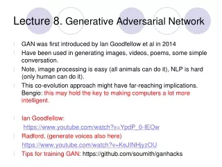
Lecture 8. Generative Adversarial Network • GAN was first introduced by Ian Goodfellow et al in 2014 • Have been used in generating images, videos, poems, some simple conversation. • Note, image processing is easy (all animals can do it), NLP is hard (only human can do it). • This co-evolution approach might have far-reaching implications. Bengio: this may hold the key to making computers a lot more intelligent. • Ian Goodfellow: https://www.youtube.com/watch?v=YpdP_0-IEOw • Radford, (generate voices also here) https://www.youtube.com/watch?v=KeJINHjyzOU • Tips for training GAN: https://github.com/soumith/ganhacks
Autoencoder As close as possible NN Encoder NN Decoder code NN Decoder Randomly generate a vector as code Image ? code
Autoencoder with 3 fully connected layers Training: model.fit(X,X) Cost function: Σk=1..N (xk – x’k)2 Large small, learn to compress
Auto-encoder 2D code NN Decoder NN Decoder code -1.5 1.5 NN Decoder
Auto-encoder -1.5 1.5
Auto-encoder NN Encoder NN Decoder input output code VAE Minimize reconstruction error m1 m2 NN Encoder m3 c1 NN Decoder input output + c2 exp σ1 c3 σ2 σ3 ci = exp(σi)ei + mi X e1 From a normal distribution Minimize e2 e3 Σi=1..3 [exp(σi)−(1+σi)+(mi)2 ] Auto-Encoding Variational Bayes, https://arxiv.org/abs/1312.6114 This constrains σi approacing 0 is good
Problems of VAE • It does not really try to simulate real images code Output NN Decoder As close as possible One pixel difference to the target Also one pixel difference to the target Fake Realistic VAE treats these the same
Gradual and step-wisegeneration NN Generator v3 NN Generator v2 NN Generator v1 Discri-minator v3 Discri-minator v2 Discri-minator v1 Generated images These are Binary classifiers Real images:
GAN – Learn a discriminator NN Generator v1 Randomly sample a vector 0 0 0 0 Something like Decoder in VAE 1 1 1 1 Discri-minator v1 image 1/0 (real or fake) Real images Sampled from DB:
Randomly sample a vector GAN – Learn a generator NN Generator v1 Train this Updating the parameters of generator v2 The output be classified as “real” (as close to 1 as possible) They have Opposite objectives Generator + Discriminator = a network Discri-minator v1 Do not Train This Using gradient descent to update the parameters in the generator, but fix the discriminator 1.0 0.13
Generating 2nd element figures You can use the following to start a project (but this is in Chinese): Source of images: https://zhuanlan.zhihu.com/p/24767059 From Dr. HY Lee’s notes. DCGAN: https://github.com/carpedm20/DCGAN-tensorflow
GAN– generating 2nd element figures 100 rounds This is fast, I think you can use your CPU
GAN– generating 2nd element figures 1000 rounds
GAN– generating 2nd element figures 2000 rounds
GAN– generating 2nd element figures 5000 rounds
GAN– generating 2nd element figures 10,000 rounds
GAN– generating 2nd element figures 20,000 rounds
GAN– generating 2nd element figures 50,000 rounds
Next few images from Goodfellow lecture Traditional mean-squared Error, averaged, blurry
256x256 high resolution picturesby Plug and Play generative network
Deriving GAN • During the rest of this lecture, we will go thru the original ideas and derive GAN. • I will avoid the continuous case and stick to simple explanations.
Maximum Likelihood Estimation • Give a data distribution Pdata(x) • We use a distribution PG(x;θ) parameterized by θ to approximate it • E.g. PG(x;θ) is a Gaussian Mixture Model, where θ contains means and variances of the Gaussians. • We wish to find θ s.t. PG(x;θ) is close to Pdata(x) • In order to do this, we can sample {x1,x2, … xm} from Pdata(x) • The likelihood of generating these xi’s under PG is L= Πi=1…m PG(xi; θ) • Then we can find θ* maximizing the L.
KL (Kullback-Leibler) divergence • Discrete: DKL(P||Q) = ΣiP(i)log[P(i)/Q(i)] • Continuous: DKL(P||Q) = p(x)log [p(x)/q(x)] • Explanations: Entropy: - ΣiP(i)logP(i) - expected code length (also optimal) Cross Entropy: - ΣiP(i)log Q(i) – expected coding length using optimal code for Q DKL= ΣiP(i)log[P(i)/Q(i)] = ΣiP(i)[logP(i) – logQ(i)], extra bits JSD(P||Q) = ½ DKL(P||M)+ ½ DKL(Q||M), M= ½ (P+Q), symmetric KL * JSD = Jensen-Shannon Divergency ∞ −∞
Maximum Likelihood Estimation θ* = arg maxθ Πi=1..mPG(xi; θ) arg maxθlog Πi=1..mPG(xi; θ) = arg maxθ Σi=1..m log PG(xi; θ), {x1,..., xm} sampled from Pdata(x) = arg maxθ Σi=1..m Pdata(xi) log PG(xi; θ) --- this is cross entropy ≅ arg maxθ Σi=1..m Pdata(xi) log PG(xi; θ) - Σi=1..m Pdata(xi )logPdata(x i) = arg minθ KL (Pdata(x) || PG(x; θ)) --- this is KL divergence Note: PG is Gaussian mixture model, finding best θ will still be Gaussians, this only can generate a few blubs. Thus this above maximum likelihood approach does not work well. Next we will introduce GAN that will change PG, not just estimating PG is parameters We will find best PG , which is more complicated and structured, to approximate Pdata.
Thus let’s use an NN as PG(x; θ) PG(x,θ) Pdata(x) G θ Prior distribution of z Smaller dimension Larger dimension How to compute the likelihood? PG(x) = Integrationz Pprior(z) I[G(z)=x]dz https://blog.openai.com/generative-models/
Basic Idea of GAN • Generator G • G is a function, input z, output x • Given a prior distribution Pprior(z), a probability distribution PG(x) is defined by function G • Discriminator D • D is a function, input x, output scalar • Evaluate the “difference” between PG(x) and Pdata(x) • In order for D to find difference between Pdata from PG, we need a cost function V(G,D): G*=arg minGmaxDV(G,D) Note, we are changing distribution G, not just update its parameters (as in the max likelihood case). Hard to learn PG by maximum likelihood
Basic Idea G* = arg minGmaxD V(G,D) Pick JSD function: V = Ex~P_data [log D(x)] + Ex~P_G[log(1-D(x))] Given a generator G, maxDV(G,D) evaluates the “difference” between PG and Pdata Pick the G s.t. PG is most similar to Pdata V(G3,D) V(G1,D) V(G2,D) G1 G2 G3
MaxDV(G,D), G*=arg minGmaxDV(G,D) • Given G, what is the optimal D* maximizing • Given x, the optimal D* maximizing is: f(D) = alogD + blog(1-D) D*=a/(a+b) V = Ex~P_data [log D(x)] + Ex~P_G[log(1-D(x))] = Σ [ Pdata(x) log D(x) + PG(x) log(1-D(x) ] Thus: D*(x) = Pdata(x) / (Pdata(x)+PG(x)) Assuming D(x) can have any value here
maxDV(G,D), G* = arg minGmaxD V(G,D) D1*(x) = Pdata(x) / (Pdata(x)+PG_1(x)) D2*(x) = Pdata(x) / (Pdata(x)+PG_2(x)) “difference” between PG1 and Pdata V(G1,D*1) V(G1,D) V(G3,D) V(G2,D)
maxDV(G,D) V = Ex~P_data [log D(x)] + Ex~P_G[log(1-D(x))] maxD V(G,D) = V(G,D*), where D*(x) = Pdata / (Pdata + PG), and 1-D*(x) = PG / (Pdata + PG) = Ex~P_data log D*(x) + Ex~P_G log (1-D*(x)) ≈ Σ [ Pdata (x) log D*(x) + PG(x) log (1-D*(x)) ] = -2log2 + 2 JSD(Pdata || PG ), JSD(P||Q) = Jensen-Shannon divergence = ½ DKL(P||M)+ ½ DKL(Q||M) where M= ½ (P+Q). DKL(P||Q) = Σ P(x) log P(x) /Q(x)
Summary: V = Ex~P_data [log D(x)] + Ex~P_G[log(1-D(x))] • Generator G, Discriminator D • Looking for G* such that • Given G, maxDV(G,D) = -2log2 + 2JSD(Pdata(x) || PG(x)) • What is the optimal G? It is G that makes JSD smallest = 0: PG(x) = Pdata (x) G* = arg minGmaxD V(G,D)
Algorithm G* = arg minGmaxD V(G,D) L(G), this is the loss function • To find the best G minimizing the loss function L(G): θG θG =−η L(G)/ θG , θG defines G • Solved by gradient descent. Having max ok. Consider simple case: f(x) = max {D1(x), D2(x), D3(x)} If Di(x) is the Max in that region, then do dDi(x)/dx D1(x) D3(x) D2(x) dD3(x)/dx dD1(x)/dx dD2(x)/dx
G* = arg minGmaxD V(G,D) Algorithm L(G) • Given G0 • Find D*0 maximizing V(G0,D) V(G0,D0*) is the JS divergence between Pdata(x) and PG0(x) • θG θG −ηΔV(G,D0*) / θG Obtaining G1(decrease JSD) • Find D1* maximizing V(G1,D) V(G1,D1*) is the JS divergence between Pdata(x) and PG1(x) • θG θG −η ΔV(G,D1*) / θG Obtaining G2(decrease JSD) • And so on …
In practice … V = Ex~P_data [log D(x)] + Ex~P_G[log(1-D(x))] • Given G, how to compute maxDV(G,D)? • Sample {x1, … ,xm} from Pdata • Sample {x*1, … ,x*m} from generator PG Maximize: V’ = 1/m Σi=1..m logD(xi) + 1/m Σi=1..m log(1-D(x*i)) Positive example D must accept Negative example D must reject This is what a Binary Classifier do Output is D(x) Minimize Cross-entropy If x is a positive example Minimize –log D(x) If x is a negative example Minimize –log(1-D(x))
Binary Classifier Output is f(x) Minimize Cross-entropy D is a binary classifier (can be deep) with parameters θd {x1,x2, … xm} from Pdata (x) Positive examples {x*1,x*2, … x*m} from PG(x) Negative examples L = - V’ Minimize or If x is a positive example Minimize –log f(x) • V’ = Σi=1..m logD(xi) + 1/m Σi=1..m log(1-D(x*i)) Maximize If x is a negative example Minimize –log(1-f(x))
Initialize θd for D and θg for G Algorithm Can only find lower bound of JSD or maxDV(G,D) Ian Goodfellow comment: this is also done once • In each training iteration • Sample m examples {x1,x2, … xm} from data distribution Pdata(x) • Sample m noise samples {z1, … , zm} from a simple prior Pprior(z) • Obtain generated data {x*1, … , x*m}, x*i=G(zi) • Update discriminator parameters θd to maximize • V’ ≈ 1/m Σi=1..m logD(xi) + 1/m Σi=1..m log(1-D(x*i)) • θd θd + ηΔV’(θd) (gradient ascent) • Simple another m noise samples {z1,z2, … zm} from the prior Pprior(z),G(zi)=x*i • Update generator parameters θg to minimize V’= 1/mΣi=1..m logD(xi) + 1/m Σi=1..m log(1-D(x*i)) θg θg − ηΔV’(θg) (gradient descent) Learning D Repeat k times Learning G Only Once
Objective Function for Generatorin Real Implementation V = Ex~P_data [log D(x) + Ex~P_G[log(1-D(x))] Training slow at the beginning V = Ex~P_G [ − log (D(x)) ] Real implementation: label x from PG as positive
Some issues in training GAN M. Arjovsky, L. Bottou, Towards principled methods for training generative adversarial networks, 2017.
Evaluating JS divergence Discriminator is too strong: for all three Generators, JSD = 0 Martin Arjovsky, Léon Bottou, Towards Principled Methods for Training Generative Adversarial Networks,2017, arXiv preprint
Evaluating JS divergence https://arxiv.org/abs/1701.07875 • JS divergence estimated by discriminator telling little information Weak Generator Strong Generator
Discriminator 1 for all positive examples 0 for all negative examples • V = Ex~P_data [log D(x)] + Ex~P_G[log(1-D(x))] • = 1/m Σi=1..m logD(xi) + 1/m Σi=1..m log(1-D(x*i)) maxDV(G,D) = -2log2 + 2 JSD(Pdata || PG ) = 0 log 2 when Pdata and PG differ completely Reason 1. Approximate by sampling Weaken your discriminator? Can weak discriminator compute JS divergence?
Discriminator GAN implementation estimation 1 0 • V = Ex~P_data [log D(x)] + Ex~P_G[log(1-D(x))] • = 1/m Σi=1..m logD(xi) + 1/m Σi=1..m log(1-D(x*i)) ≈ 0 maxDV(G,D) = -2log2 + 2 JSD(Pdata || PG ) = 0 log2 Theoretical estimation Reason 2. the nature of data Pdata(x) and PG(x) have very little overlap in high dimensional space
Evolution http://www.guokr.com/post/773890/ Better
Evolution needs to be smooth: JSD(PG_0 || Pdata) = log2 PG_0(x) Pdata(x) …… Better PG_50(x) Pdata(x) JSD(PG_50 || Pdata) = log2 Not really better …… …… PG_100(x) Pdata(x) JSD(PG_100 || Pdata) = 0
One simple solution: add noise • Add some artificial noise to the inputs of discriminator • Make the labels noisy for the discriminator • Discriminator cannot perfectly separate real and generated data Pdata(x) and PG(x) have some overlap Noises need to decay over time