Download
1 / 32
320 likes | 375 Vues
Delve into the study of gene frequencies and evolution with Population Genetics, ranging from Hardy-Weinberg’s law to practical applications like DNA fingerprinting and conservation efforts. Understand how genetic polymorphisms shape populations and the impact of evolutionary forces. Discover the theoretical foundations provided by notable figures like Darwin, Mendel, Fisher, and more. Explore themes such as mutations, allele frequencies, and the forces influencing genetic traits. Unravel the significance of Hardy-Weinberg equilibrium and the fundamental assumptions underlying this law.

E N D
Population genetics concerns the study of gene frequencies and their variation in time and space. In other words; the study of evolution. Population genetics includes a qualitative branch (treating traits determined by genes at single loci) and a quantitative branch (treating traits influenced by genes at many loci (breeding genetics). The most sentral theoreme is Hardy-Weinberg’s law, which in a sense is the "population version" of the Mendelian laws of inheritance. The materials studied are genetic polymorfisms, and the methods leans heavily towards mathematical models and statistics tools. Our starting question is: How are the gene (allele) frequencies in populations influenced by the 4 evolutionary forces [mutations, genetic drift, gene flow (immigration), and selection]. BI 3010 H08 Population genetics Halliburton Kap 1-3
BI 3010 H08 Population genetics Halliburton Kap 1-3 Genetic nomenclature (jargon): Synonyms: Gene frequency = allele frequency = allelic proportion The frequency of an allele (e.g. A,B,C) is often abbreviated qA, qB, qC, etc, or alternatively, pA, qB, rC etc. In general, the phenotypes (e.g. active isozymes, proteins) are written in normal font (e.g. AA phenotype) while genotype is written in Italic (AA genotype). However, there is no general consistency between textbooks in how this is handled.
BI 3010 H08 Population genetics Halliburton Kap 1-3 Population genetics is in itself a theoretical science based on mathematical models and statistic analyses. However, it has a wide range of practical applications, such as: • Plant- and animal breeding • DNA fingerprinting in forensic science • Habitat fragmentation and conservation of endangered species • Understanding the mechanisms of genetic differentiation and speciation • HUGO (the Human Genome Project) • Identification of genes related to disease in humans • The ancient history and evolution in man • Estimating effects of releasing GMO in nature • Identification and delimitation of biological units in resource management
BI 3010 H08 Population genetics Halliburton Kap 1-3 • The theoretical foundation was laid down by a.a.: • Charles Darwin (natural selection theory) • Gregor Mendel (pea crossings and segregation ratios) • Hardy and Weinberg (HW-principle) [no photo] • Ronald A. Fisher (Anova; Analysis of Variance) • Sewall Wright (shifting balance, adaptive landscapes, FST, inbreeding coeff.) • Theodosius Dobzhansky (Drosophila, speciation, hybrides/backcrossing) • Richard Lewontin (elektrophoresis as a tool) • Masatoshi Nei (genetic distance, (GST (multilocus FST)) • Motoo Kimura (neutral theory of genetic differentiation and evolution)[no photo]
Types of genetic polymorphisms Variation within and between populations Variation in qualitative and quantitative traits Variation due to sexual reproduction 5. How are new traits formed? 6. Adaptive landscapes 7. Interaction between the four evolutionary forces 8. Speciation; it's genetic basis BI 3010 H08 Population genetics Halliburton Kap 1-3 Some important themes:
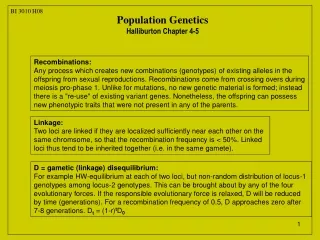
Population genetics Halliburton Kap 1-3 BI 3010 H08 • Populations are the real evolutionary units. • The raw material of evolution are mutations, which can accumulate with time • in populations and species, and result in multiple alleles at many loci. • Evolution can thus be defined as "any change in allele frequencies". • The frequencies of different alleles at a locus can be changed by the • 4 evolutionary forces, which are: • Mutations • Random genetic drift • Gene flow (immigration) • Selection • If these forces are nullified, we have what is called a "Hardy-Weinberg population"; a panmictic (random mating), • statistically ideal population where the allele frequencies, and thereby the genotype frequencies, are constant and • do not change over generations (a socalled H-W equilibrium). The population genetic approach is to assume a • H-W equilibrium situation, and then study how the 4 evolutionary forces each, and in combinations, influence the • allele- and genotypic frequencies within and between • populations.
BI 3010 H08 Population genetics Halliburton Kap 1-3 • Underlying assumptions for the H-W law about the relation between • allele frequencies and genotypic proportions: • Panmixi (random mating) • No mutations • No random genetic drift (i.e. infinitely large population) • No gene flow between populations (i.e. no immigration) • No selection (same fitness for all genotypes)
BI 3010 H08 Population genetics Halliburton Kap 1-3 The Hardy-Weinberg law: "In a panmictic, statistically ideal population, the genotypic proportions is determined by the allele frequencies (p and q in formula I below) at the locus according to the binomial formula". [multinomial if more than two alleles; e.g. 3 in formula II)] I(p+q)2 = p2 + 2pq + q2 (if only two alleles) II (p+q+r)2 = p2 + 2pq + 2pr + q2 + 2qr + r2 (if 3 alleles) [ The number of possible genotypes is n(n+1)/2 where n=number of alleles ] The allele frequencies will be constant over generations and restore the same genotypic proportions in each new generation. Allele- and genotype frequencies can thus serve as population characteristics.
Population genetics Halliburton Kap 1-3 BI 3010 H08 Methods for the study of frequencies of single genes
BI 3010 H08 Population genetics Halliburton Kap 1-3 separation page
BI 3010 H08 Population genetics Halliburton Kap 1-3 Chi-squared ( 2 ) test for goodness-of-fit to H-W proportions Assume that we have studied a locus with two alleles by electrophoresis. We have named the alleles F and S according to their electrophoretic migration distance (Fast and Slow). There are three possible genotypes (FF, SF og SS). In a sample of N=50 individuals from a natural population we observed 10 with genotype FF, 28 with genotype SF, and 12 with genotype SS. We want to test if this genotype distribution is reasonably close to the H-W expected values calculated from the observed allele frequencies in the sample. For this we use a so-called chi-squared Goodness-of-fit test (table below). We use a table of critical values of the chi-square distribution in some text book to check the significance level P of the chi-square value calculated. The degrees of freedom (df) is caclulated as the number of genotypes minus the number of alleles (i.e. df = 3-2 =1).
Population genetics Halliburton Kap 1-3 BI 3010 H08 Critical values of the 2 distribution
BI 3010 H08 Population genetics Halliburton Kap 1-3 Effects of deviations from the assumptions of the H-W law
BI 3010 H08 Population genetics Halliburton Kap 1-3 1. Effect from the assumption of panmixia (random mating) Deviations from random mating accur in natural populations. The most common effect of non- random mating is an increase in homozygosity ( = reduced heterozygosity) in the population compared to the expected value under H-W equilobrium. Per definition this is inbreeding. The probability for homozygosity by inheritance is called the Inbreeding coefficient. (jfr path-analysis in Fig. 24-6 and Box 24-5). In principle two types of situations: a) – related individuals prefer each other or avoid each other. If two parents are more related than the average in the population, inbreeding is taking place. If less related than the average, we have outbreeding. b) – Phenotypically similar individuals for a specific trait (which have a genetic component) prefer each other at mating. Examples of this in humans can be skin colour or body length (too many homozygotes is formed each generation compared to H-W expectations. This is called positive assortative mating, and will increase the inbreeding for the trait. The opposite tendency, negative assortative mating, will increase outbreeding (reduce inbreeding) for the trait in the population.
BI 3010 H08 Populasjonsgenetikk Halliburton Kap 1-3 2. Effect of deviation from the assumption of no mutation Point mutations (basepair changes which cause amino acid substitutions) are the real source of genetic variation, and the raw material of evolution. They occur randomly but with an average frequency which appears to vary between loci. However, it is difficult to evaluate how large (or small) the difference betwen loci is. For example, mutations in particularly important proteins (or parts of proteins) will less likely ”survive” until they can be detected in a functional phenotype. This would lead to an under- estimation of the true mutation rate at such loci. However, mutation rates are for the most so low that they rarely interfere with the practical application of the Hardy-Weinberg principle on natural populations, e.g. the use of observed allele frequency to characterize populations. With respect to loss of genetic variability due to random genetic drift in isolated populations, mutations can reduce or prevent such loss. As a rule of thumb, the mutation rate ( µ ) and the population size N must satisfy the following equiation in order for level of genetic variation to be maintained: N µ≥1 If the mutation rate is 0.000001, the effective population size must thus be at least one million to prevent that the loss by genetic drift (measured as lowered heterozygosity) is not larger than the gain by new mutations.
BI 3010 H08 Population genetics Halliburton Kap 1-3 3. Effect of deviation from no random genetic drift (i.e. infinitely large population size) It can be useful to look at sexual reproduction as a process where eggs and sperm from all potential parents are coloured marbles in a bucket. They are then drawn two by two to determine each offspring's genotype at a specific locus. If all matings give the same number of offspring the frequency of each allele in the offspring (F1) generation will tend to be the same as in the parental generation (P0). However, the individuals which become parents are usually a subsample of the whole gene pool, which introduces an inaccuracy on their representability for the population. Repeated subsampling may give different outcomes although their mean in a large number of outcomes is expected to be equal to the parent generation's allele frequencies. Mathematically this process is called binomial sampling (when two alleles), and the spread around the mean frequency is called the binomial variance [(p(1-p)/2N in the formula below]. The Standard Error (SE) for an allele frequency p in the F1 generation is the square root of the binomial variance and hence calculated as: which shows that both the allele frequency and the mating population size have effect on the stability (or the variability) of allele frequencies over generations. The formula shows that allele frequencies (particularly those around 0.5) in small populations will tend to fluctuate considerably between generations. This phenomenon is called random genetic drift.
BI 3010 H08 Evolutionary forces: Examples Drosophila sp.: Genetic drift. Ne = 16 (8 males & 8 females) Random drift of allele frequencies during 19 generations in a large set of small populations (effective population size (Ne) is 16 individuals) of the fruit fly Drosophila sp. The locus under study had two alleles at intermediate allele frequencies in all populations at the start of the experiment. The portion of populations which become fixed for one or the other of the two alleles increased steadily with time.
BI 3010 H08 Population genetics Halliburton Kap 1-3 4. Effect of deviation from the assumption of no gene flow (no immigration) Immigrants from populations with different allele frequencies will (when genetically effective) cause disturbance to the stability of the local H-W frequencies. The frequencies in the local population (the recipient) will change towards that of the immigrant (the donor), to a degree that is proportional to the relative number of immigrants. The effect will accumulate over generations. Let the local allele frequency be p and that of the immigrant q. If the immigrant constitute a proportion m in the local reproduction, the change in local allele frequency is described by: p = m(q-p) which shows that the amount of change depends both on the relative number of immigrants and on the difference in allele frequency between donor and recipient. This change will, according to H-W, result in a change in local genotypic proportions as well. Sometimes a sample may contain a physical mixture of individuals from two or more populations with different allelic and genotypic frequencies. When counting up genotypes in such a mixture there will be too few heterozygotes compared to what is expected from the allele frequencies and the H-W law. This phenomenon (i.e. the deficiency) is called the "Wahlund effekt", and is actually a tool for detecting such physical mixtures. The magnitude of the deficiency is positively correlated with the difference in allele frequencies and the relative size of the involved groups. With respect to genetic differentiation between populations, immigration (gene flow) will counteract the effect of genetic drift in local populations. As a rule-of-thumb, the magnitude of immigration sufficient to counteract substantial local genetic differentiation must in each generation be: m≥ 1 / N which, re-arranged as mN ≥ 1, shows that it is in fact the absolute number of immigrants (Nm) which is important (because it is the differentiating effect of genetic drift which is to be counteracted, and that effect is largest when N is small and vice versa). However, even though an immigration of one individual per generation is sufficient to counteract fixations of different alleles in the populations, it will not prevent that substantial differences in allele frequencies can arise and sustain between populations.
BI 3010 H08 Population genetics Halliburton Kap 1-3 5. Effect of deviation from the assumption of no selection Selection is capable of causing large changes in allele frequencies between generations, and give rise to genotypic proportions that deviate substantially from H-W expectations. In order to treat selection, we shall first define and show how to estimate two different population parametres, the fitness-coefficient (w) and the selection coefficient (s). For this purpose we assume a very simple scenario with three genotypes at one locus, and fitness calculated from relative survival only (there are of course many other possible components in individual fitness). On this locus, we count the number of the different genotype before and after selection (e.g. by birth and just before reproducion). Cf table next page.
BI 3010 H08 Population genetics Halliburton Kap 1-3 Box 1 Selection Calculation of fitness- and selection coefficients for survival (i.e. partial coeffs.) The table shows an example of selection of the type called "Balanced selection" or "Balanced polymorphism", or "Overdominance", in which the heterozygote has the highest fitness coefficient (survives best).
BI 3010 H08 Population genetics Halliburton Kap 1-3 Selection con't. The efficiency of selection, measured as the change in allele frequency per generation, depends not only on the size of the selection coefficients, but also on the allele frequency itself (the change per generation is largest for allele frequencies around 0.5). This can be seen from the formula for the average fitness for the population for a single locus trait, where the allele frequencies are incorporated as follows: Wmean = p2WFF + 2pqWFS + q2WSS From this formula we can derive the "mean fitness" for each allele as: WF-mean = pWFF + qWFS, and WS-mean = pWFS + qWSS After some algebra the above formulas can be combined to give p; the change in allele frequency per generation due to selection: p = pq[WF-mean – WS-mean] / Wmean which states that the speed of change in allele frequency per generation is proportional to the frequency (pq) of heterozygotes, which in turn is largest at allele frequencies around 0.5. At extreme allele frequencies (approaching 0 or 1), the change per generation will be small.
BI 3010 H08 Population genetics Halliburton Kap 1-3 The three main type of selection: Selection is often divided in three types based on the effect is has on the genotypic and allelic frequencies at a locus (or on the mean value and variance for quantitative traits). 1. directional selection 2. stabilizing selection 3. disruptive selection
BI 3010 H08 Population genetics Halliburton Kap 1-3 Relevant computer simulations of the effect of selection on population allele frequencies can be performed e.g. with the PopG.exe Windows programme, or alternatively with the P14.exe DOS programme available at It's learning. The following slides are made with the latter.
BI 3010 H08 Population genetics Halliburton Kap 1-3 Type 1: Directional selection (single locus):
BI 3010 H08 Population genetics Halliburton Kap 1-3 Type 2: Stabilizing selection (balanced polymorphism, overdominance)
BI 3010 H08 Population genetics Halliburton Kap 1-3 Type 3: Disruptive selection (underdominance)
BI 3010 H08 Population genetics Halliburton Kap 1-3 A well-known example of a balanced polymorphism: The maps show the similarity of the geographical distribution of the human haemoglobin allele causing sickle-cell anemia, and the distribution of the malaria blood parasite.
Population genetics Halliburton Kap 1-3 Box 2 BI 3010 H08 Chi-squared test of genetic differences between samples To test for differences in allelic or genotypic proportions between samples we use an RxC (rows by columns) chi-square contingency test. We usually test for both genotypic and allelic heterogeneity between samples. The latter is statistically the most powerfulI one. Consider two samples of N=100 each, and one polymorphic locus with two alleles (A og B): Genotypes_______ Samples AA AB BB N ------------------------------------------------------------------------------------------------- Sample 1 36 (26) 48 (48) 16 (26) 100 Sample 2 16 (26) 48 (48) 36 (26) 100 ------------------------------------------------------------------------------------------------- Total 52 96 52 200 ======================================================= Our "Null hypothesis" for test is that the samples are drawn from one and the same population. If so, our best estimate of the true genotype and allele distribution in the materials is found in the "Total". We therefore use the distribution in the "Total" to estimate what "should have been" in the two single samples (we "forget" about the H-W distributions in this test).The expected number of AA genotypes in Sample 1 is then, e.g., ((52/200)*100)=26. As in all chi-square tests we find the test observator in this way: Take the square of the difference between observed and expected value, and divide it by the expected value. Do this for all genotypes in both samples, and sum the results. The number of degrees of fredom in a contingency table (RxC) is calculated differently from the "H-W Goodness-of-fit". Degrees of fredom is here calculated as (R-1)(C-1). For the genotypic values in the table above, we find a chi-square value of 15.38, and 2 degrees of freedom. In a textbook table of the chi-square distribution we find that this corresponds to a significance level of P < 0.001. (actually the exact P-value is 0.00046). For testing for homogeneity of allelic proportions in the same two samples, the RxC table will look like this: Allele _ Sample A B N ------------------------------------------------------------------------------------------------- Sample 1 120 (100) 80 (100) 200 Sample 2 80 (100) 120 (100) 200 ------------------------------------------------------------------------------------------------- Total 200 200 400 ======================================================= The chi-square for this table is 16.00. However, here we have only one degree of freedom. Therefore the P-value for this outcome (P=0.00006) is lower than in the genotype test. In both tests, the null hypothesis can be safely rejected. Our samples are not drawn from the same population.
BI 3010 H08 Population genetics Halliburton Kap 1-3 Genetic differentiation and genetic structure Sewall Wright’s Fst (a relative measure of differentiation): Evolution can be defined as any change in population allele frequencies. The evolutionary forces that can bring about allele frequency changes (mutations, random genetic drift, gene flow, and selection) can, given time, lead to different allele frequencies in the populations. Several models have been suggested to describe this process. One of the best known and most frequently employed is Sewall Wright's "Mainland-Island" model. It assumes a start ("Mainland") population which is split in a large number of sub-populations ("Island populations"), and describes the genetic differentiation which takes between these in formulas which considers e.g. sub-population sizes, migration rates, and number of generations. Wright uses a specific measure – FST – for the degree of differentiation. The calculation of FST is based on heterozygosities (H), which can be calculated for groups at different hierarchical levels (sub- and total population). The observed heterozygosity (HO) at a locus in a group is simply the proportion of heterozygote genotypes, while the expected heterozygosity is calculated from the allele frequencies assuming H-W equilibrium (HE = 1- xi2). The calculated average H at a locus is usually denoted with a "bar" above it, and is the arithmetic mean of H at all included loci (monomorphic as well as polymorphic): Fst = 1 - [Hmean / Htotal ] where Hmean is the arithmetic mean of the single locus heterozygosities in all subpopulations, while Htotal is the expected (H-W) heterozygosity based on the joint allele frequency in the total material. It is apparent that Fst is 0 when all the subpopulations are genetically identical, and 1 when they are fixed for different alleles. Masatoshi Nei suggested later an analogous measure (GST) which can be calculated fro sample allele frequencies rather than genotype frequencies, assuming that all sub-populations are in H-W equilibrium. GST can be calculated as a mean over many loci. Nei’s I and D (absolute measures of genetic similarity and differentation): Masatoshi Nei also suggested another measure, D, (“Genetic Distance”), which gives an estimate of the absolute genetic differences between taxa (" the mean number of amino acid substitutions per locus"). This measure utilises allele frequencies at many loci, and is calculated for each locus via the quantity I ("Genetic Identity") according to this formula: I = xiyi / SQRT[ (xi2)(yi2)], and so D = - ln(I) where xi and yi are frequency of the i-th allele in population X and Y, respectively (SQRT means "square root"). The overall D is calculated as the arithmetic mean over the actual number of loci genotyped.
BI 3010 H08 Practical calculation of FST from genotype data Population genetics Halliburton Kap 1-3 Box 3 Consider a number of samples from different parts of the distribution area of a species. By electrophoretic analyses the individual genotypes at a particular locus are determined. This locus has two alleles A and B| which segregates in three genotypes AA, AB, and BB. After the analyses the follwing table can be constructed (only the FST relevant figures are included). Samples AA AB BB N qA qB H ------------------------------------------------------------------------------------------------------------------------------------------------------------------ Sample 1 17 46 37 100 .46 Sample 2 89 62 9 160 .39 Sample3 48 104 48 200 .52 ------------------------------------------------------------------------------------------------------------------------------------------------------------------ Mean Hobs .46 ------------------------------------------------------------------------------------------------------------------------------------------------------------------ Total 154 212 94 460 .57 .43 .49 ============================================================================================ Mean observed heterozygosity (Hmean) for the three samples is calculated as [( 0.46+0.39+0.52 ) / 3)], giving 0.46. Expected (Hardy-Weinberg) heterozygosity in the total material (Htotal) is calculated based on the allele frequencies, and is in this case: (2*0.57*0.43 =) 0.49. Fst = 1 - Hmean / Htotal Inserting these values in the formula gives in this case an FST value of [ 1 – (.46/.49) ] = 0.06. The measure, FST,comes from a decomposition of the total genetic heterogeneity into a "within" and a "between" component. In this example, 6% (i.e. fraction 0.06) of the total genetic heterogeneity is due to differences between samples. The rest (94%) of the heterogeneity is found within samples (i.e. between individuals). The calculations above follow Sewall Wright's original concept for one locus. For multi-locus calculations (e.g. Nei's GST) one uses the expected (i.e. not observed) heterozygosity both for sub-samples and the total. Masatoshi Nei's G-statistics (GST) is an extension of FST to many alleles and many loci. The main difference in calculation is that it uses HW-expected heterozygosities in the subpopulations (here: samples). The overall GST is calculated as the average over all loci.
BI 3010 H08 Population genetics Halliburton Kap 1-3 Useful software: Hweq2.exe (Hardy-Weinberg chi-square goodness-of-fit test. 2 alleles, 3 genotypes) ChiRxC.exe (chi-square contingency table test; Rows by Columns) PopG.exe (interactive simulation of evolutionary forces, graphic display) -------------------- These programmes will be uploaded to It’s learning
BI 3010 H08 Population genetics Halliburton Kap 1-3 Last slide