Download

1 / 50
510 likes | 570 Vues
Quick sort is a powerful sorting algorithm that partitions an array based on a pivot element. By recursively sorting subarrays, Quick Sort achieves efficient sorting. The algorithm's best and worst-case analyses reveal its effectiveness.

E N D
Design and Analysis of Algorithms TE IT Mrs. U. M. Kalshetti
Divide and Conquer Algorithms – Quick Sort • Quick sort is one of the most powerful sorting algorithm. • Quick sort works by finding an element, called the pivot, in the given input array and partitions the array into three sub arrays such that • The left sub array contains all elements which are less than or equal to the pivot • The middle sub array contains pivot • The right sub array contains all elements which are greater than or equal to the pivot • Now the two sub arrays, namely the left sub array and the right sub array are sorted recursively
Quick Sort • Quick Sort: • To sort the given array a[1…n] in ascending order: 1. Begin 2. Set left = 1, right = n 3. If (left < right) then 3.1Partition a[left…right] such that a[left…p-1] are all less than a[p] and a[p+1…right] are all greater than a[p] 3.2Quick Sort a[left…p-1] 3.3Quick Sort a[p+1…right] 4. End
Quick Sort • To partition the given array a[1…n] such that every element to the left of the pivot is less than the pivot and every element to the right of the pivot is greater than the pivot. 1. Begin 2. Set left = 1, right = n, pivot = a[left], p = left 3. For r = left+1 to right do 3.1If a[r] < pivot then 3.1.1a[p] = a[r], a[r] = a[p+1], a[p+1] = pivot 3.1.2Increment p 4. End with output as p
Analysis of Partition algorithm • Inside the ‘For’ loop, there is one comparison statement. • Number of times the comparison statement will gets executed = n-1 • Worst case complexity is O( n ) • Also, since the complexity is O(n), the number of times the comparison • Statement will gets executed = c. n where c is a constant.
Analysis of Quick Sort • Quicksort is recursive. • The best / worst case is calculated based on the selection of the pivot. • If the pivot selected happens to be the median of the elements, then best case will happen. • If the pivot is always the smallest, then worst case will happen. • The pivot selection takes c.N amount of time. • Running time = running time of two recursive calls + time spent on partition. • T(n) = T(i) + T(N- i -1) + c.N • T(0) = T(1) = 1
Analysis of Quick Sort • Best Case Analysis: • If the pivot happens to be the median then is the best case. • The partition algorithm splits the array into 2 equal sub arrays. • The complexity of the partition algorithm is O(n). So we are taking it as c.n, where c is a constant. • T(n) = 2T(n/2) + c n • Divide both sides by n • T(n) / (n) = T(n/2) / (n/2) + c • T(n/2) / (n/2) = T(n/4) / (n/4) + c • T(n/4) / (n/4) = T(n/8) / (n/8) + c • … • T(2)/2 = T(1) / (1) + c • T(n) / (n) = T(1) / (1) + c log n • T(n) = c nlog n + n • T(n) = O(n log n)
Analysis of Quick Sort • Worst Case Complexity: • The pivot is always the smallest element or the biggest element. • So, here i = 0 • T(n) = T(n-1) + c.n, n > 1 • T(n - 1)=T(n - 2) + c. (n - 1) • T(n - 2)=T(n - 3) + c. (n - 2) • … • T( 2 ) = T( 1 ) + c. (2) • Here we ignore T(0) as it is insignificant. • From the above equations, • T(n) = T(1) + c. Σni=2I • T(n) = O(n2)
Greedy Method • For some problems- require n inputs and obtain a subset that satisfies some constraints • Greedy design technique is primarily used in optimizationproblems • The Greedy approach helps in constructing a solution for a problem through a sequence of steps where each step is considered to be a partial solution. • This partial solution is extended progressively to get the complete solution • The choice of each step in a greedy approach is done based on the following • It must be feasible (should satisfy problem’s constraints) • It must be locally optimal (minimize/maximize objective function) • It must be irrevocable(should not get changed in subsequent steps)
Greedy Method • General method Greedy(a,n) { // a[1..n] contains n inputs Solution0 For i=1 to n do Xselect(a) If feasible(solution,x) then solution= union(solution,x) Return solution }
Greedy Method • Solve the subproblem, find the best for that subproblem. • Solve the subproblem arising after choice is made • Choice depends on the previously made choices • Choices are made one after another reducing each given problem into smaller one hence it is called greedy.
Prim’s Algorithm • Connected graph G, root r • Vertices not in the TREE reside in a min-priority queue Q based on key field • For each vertex v, key[v] is minimum weight of edge connecting v to a vertex in the TREE • Key[v]=∞ if there is no such edge • π[v] is the parent of v in the TREE • Minimum spanning tree A A={ (v, π[v] ) : v Є V-{r} –Q } • When algorithm terminates , Q is empty, A={ (v, π[v] ) : v Є V-{r} }
Prim’s Algorithm O(V) O(log V) V O(E) Times altogether
Prim’s Algorithm • If min-priority queue is implemented as min-heap, then its time is O(logV), otherwise it is O(V). • Hence time complexity is either O(Vlog V) or O(V2). • With the assumptions– line 9 can be implemented in constant times, line 11 can be implemented as updating values in mean-heap requires O(logV) time. • Total time O(V logV + E logV)= O(E logV).
Kruskal’s Algorithm • It finds a safe edge to add to the growing forest by finding, of all the edges that connect any two trees in the forest, an edge (u ,v) of least weight.
Kruskal’s Algorithm O(ElogE) O(V) O(E)
Kruskal’s Algorithm • Running time of Kruskal’sAlgo is O(E logE) • But we have E >= V-1 and E < V2 • Hence logE < 2 logV • logE = O(logV) • Hence running time is O(ElogV)
Tower of Hanoi • There are 3 pegs • There are N disks stacked on the first peg. (The disks has a hole in the center). • Each disk has a different diameter.
Tower of Hanoi • Problem Hanoi(N): • Move the N disks from peg 1 to peg 3 • You must obey a set of rules. • Tower of Hanoi Rules: • You can only move one disk at a time (from any peg to any other peg), and • You may not stack a smaller diskon top of a larger disk
Tower of Hanoi • Move the top N - 1 disks from Src to Aux (using Dst as an intermediary peg) • Move the bottom disk from Src to Dst • Move N - 1 disks from Aux to Dst (using Src as an intermediary peg)
Tower of Hanoi Solve(N, Src, Aux, Dst) if N is 0 exit else Solve(N - 1, Src, Dst, Aux) Move from Src to Dst Solve(N - 1, Aux, Src, Dst)
Tower of Hanoi Algorithm TowerofHanoi(n,x,y,z) //Move the top n disks from tower x to tower y { If(n >= 1)then { TowerofHanoi(n-1,x,z,y); Write(“move top disk from tower”,x,”to top of tower”,y); TowerofHanoi(n-1,z,y,x); } }
Tower of Hanoi • Running time T(n)= 2 T(n-1) + 1 T(1)=1, T(2)=3, T(3)=7, T(4)=15, T(5)=31 T(n)= 2n-1 T(n)=O(2n)
Union-Find data structure • Store disjoint sets of elements that supports the following operations • makeUnionFind(S) returns a data structure where each element of S is in a separate set • find(u) returns the name of set containing element u. Thus, u and v belong to the same set iff find(u) = find(v) • union(A,B) merges two sets A and B
Union-Find data structure Algorithm SimpleUnion (i, j) // i & j are roots of sets. { p[i] = j; } Algorithm SimpleFind (i ) // return root of ‘i’ { while (p[i] >=0) do i=p[i]; return i; }
Array Representation void Union1( inti , int j ) { parent[i] = j ; } EX: S1 ∪ S2 Union1( 0 , 2 ) ; [7] [9] [2] [4] [6] [8] [3] [5] [0] [1] i -1 -1 4 0 4 -1 0 0 parent 2 2 2 EX: Find1( 5 ) ; = 2 i int Find1( inti ) { for(;parent[i] >= 0 ; I = parent[i]) ; returni ; }
Analysis Union-Find Operations • For a set of n elements each in a set of its own, then the result of the union function is a degenerate tree. • The time complexity of the following union-find operation is O(n2). • The complexity can be improved by using weighting rule for union. n-1 n-2 union(0, 1), find(0) Union operation O(n) union(1, 2), find(0) Find operation O(n2) union(n-2, n-1), find(0) 0
Union-Find data structure • If we want to perform n-1 unions then can be processed in Linear time O(n) • The time required to process a find for an element at level ‘i’ of a tree is O(i), so total time needed to process n finds is O(n^2) • We apply weighting rule for Union, which says that if the number of nodes in the tree with root i is less than the number of nodes in the tree with root j, then make j as the parent of i, otherwise make i, as the parent of j.
Union-Find data structure • Similarly we use CollapseFind , to improve the performance of find • Collapsing rule says that, if j is a node on the path from i to its root node and p[i] is not root[i], then set p[j] to root[i]
Union-Find data structure Weighted-union(I,j) { Temp=p[i]+p[j]; If(p[i]>p[j]) // i has fewer nodes { p[i]=j, p[j]=temp; } Else { p[j]=I; // j has fewer nodes p[i]=temp; } } Collapse-find(i) { r=I; While(p[r]>=0) r=p[r]; while(i=r) { s=p[i]; p[i]=r; i=s; } } Weighted-union takes O(1) time Collapse-find takes O(log n) time
i [7] [9] [2] [4] [6] [8] [1] [3] [5] [0] -1 -1 -1 -1 -1 -1 -1 -1 -1 -1 parent -2 -3 0 0 void union2 (inti, int j) { int temp = parent[i] + parent[j]; if ( parent[i]>parent[j]) { parent[i]=j; parent[j]=temp; } else { parent[j]=i; parent[i]=temp; } } unoin2 (0 , 1 ) unoin2 (0 , 2 ) unoin2 (0 , 3 ) temp = -2 temp = -3 1 0 2 3 n-1 1 1 2 1 2 3 EX: unoin2 (0 , 1 ) , unoin2 (0 , 2 ) , unoin2 (0 , 2 )
Weighted Union • Lemma 5.5: Assume that we start with a forest of trees, each having one node. Let T be a tree with m nodes created as a result of a sequence of unions each performed using function WeightedUnion. The height of T is no greater than . • For the processing of an intermixed sequence of u – 1 unions and f find operations, the time complexity is O(u + f*log u).
Trees Achieving Worst-Case Bound [-1] [-1] [-1] [-1] [-1] [-1] [-1] [-1] 0 1 2 3 4 5 6 7 (a) Initial height trees [-2] [-2] [-2] [-2] 0 2 4 6 1 3 5 7 (b) Height-2 trees following union (0, 1), (2, 3), (4, 5), and (6, 7)
Trees Achieving Worst-Case Bound (Cont.) [-8] [-4] [-4] 0 4 0 6 5 2 2 1 1 4 6 5 7 3 3 (c) Height-3 trees following union (0, 2), (4, 6) 7 (d) Height-4 trees following union (0, 4)
Collapsing Rule • Definition [Collapsing rule] • If j is a node on the path from i to its root and parent[i]≠ root(i), then set parent[j] to root(i). • The first run of find operation will collapse the tree. Therefore, all following find operation of the same element only goes up one link to find the root.
Ex: find2 (7) int find2(int i) { int root, trail, lead; for (root=i; parent[root]>=0; root=parent[root]); for (trail=i; trail!=root; trail=lead) { lead = parent[trail]; parent[trail]= root; } return root: } [-8] 0 Root 2 1 6 7 4 Trail 6 5 3 Lead 7
Analysis of WeightedUnion and CollapsingFind • The use of collapsing rule roughly double the time for an individual find. However, it reduces the worst-case time over a sequence of finds.
Dijkstra’s Algorithm Single source shortest path problem
Knapsack Problem • We are given n objects and a knapsack or bag. • Object i has a weight wi and the knapsack has a capacity m. • If a fraction xi, 0 < xi < 1, of object i is placed into the knapsack, then a profit of piXi is earned. • Objective • to obtain a filling of the knapsack that maximizes the total profit earned. • Since the knapsack capacity is m, we require the total weight of all chosen objects to be at most m.
Knapsack Problem • Consider the following instance of the knapsack problem: • n = 3,m = 20,(p1,p2,P3) = (25,24,15), and (w1,w2,w3) = (18,15,10). • Four feasible solutions are:
Void Greedy Knapsack(m,n) • //p[1:n] • //w[1:n] • //x[1:n] • { for i=1 to n do x[i]=0.0 U=m For i=1 to n do if w[i]>U break; x[i]=1.0 U=U-w[i] If i<= n x[i]=U/w[i] }
Huffman Coding • C- set of characters • c Є C c.freq is frequency of character c • |C|-1 merging operations
Huffman coding HUFFMAN(C ) 1 n =|C| 2 Q = C 3 for i = 1 to n-1 4 allocate a new node z • z.left= x = EXTRACT-MIN(Q) • z.right= y= EXTRACT-MIN(Q) • z.freq = x.freq + y.freq 8 INSERT(Q,z) 9 return EXTRACT-MIN(Q) // return the root of the tree