Practical Data Science with R - Choosing and evaluating models
270 likes | 957 Vues
Practical Data Science with R - Choosing and evaluating models. Kim Jeong Rae UOS.DML. 2014.11.3. Contents. Mapping problems to machine learning tasks Evaluating models Evaluating classification models Evaluating scoring models Evaluating probability models Evaluating ranking models

Practical Data Science with R - Choosing and evaluating models
E N D
Presentation Transcript
Practical Data Sciencewith R- Choosing and evaluating models Kim Jeong Rae UOS.DML. 2014.11.3.
Contents • Mapping problems to machine learning tasks • Evaluating models • Evaluating classification models • Evaluating scoring models • Evaluating probability models • Evaluating ranking models • Evaluating clustering models • Validating models
Mapping problems to machine learning tasks Some common Classification method
Evaluating models – classification models(1/2) spamD <- read.table('spamD.tsv',header=T,sep='\t') spamTrain <- subset(spamD,spamD$rgroup>=10) # Spliting Test/Train data spamTest <- subset(spamD,spamD$rgroup<10) # Spliting Test/Train data spamVars <- setdiff(colnames(spamD),list('rgroup','spam')) # Deleting selection columns spamFormula <- as.formula(paste('spam=="spam"', paste(spamVars, collapse=' + '), sep=' ~ ')) spamModel <- glm(spamFormula, family=binomial(link='logit'), data=spamTrain) # y={0,1} spamTrain$pred<- predict(spamModel,newdata=spamTrain, type='response') spamTest$pred <- predict(spamModel,newdata=spamTest, type='response') print(with(spamTest,table(y=spam,glmPred=pred>0.5))) sample <- spamTest[c(7,35,224,327),c('spam','pred')] print(sample) Building and applying a logistic regression spam model
Evaluating models – classification models(2/2) cM <- table(truth=spamTest$spam, prediction=spamTest$pred>0.5) print(cM) # Accuracy = (TP+TN)/(TP+FP+TN+FN) (cM[1,1]+cM[2,2])/sum(cM) # Precision = TP /(TP+FP) (cM[2,2])/(cM[2,2]+cM[1,2]) # Recall = TP /(TP+FN) (cM[2,2])/(cM[2,2]+cM[2,1]) # F1 = 2*Precision*Recall/(Precision+Recall) P <- (cM[2,2])/(cM[2,2]+cM[1,2]) R <- (cM[2,2])/(cM[2,2]+cM[2,1]) 2*P*R/(P+R) # Sensitivity(=True positive rate) = Recall # Specificity(=True negative rate) = TN/(TN+FP) (cM[1,1])/(cM[1,1]+cM[1,2]) Accuracy, Precision, Recall etc.
Evaluating models – scoring models(1/2) d <- data.frame(y=(1:10)^2, x=1:10) model <- lm(y~x, data=d) summary(model) d$prediction <- predict(model, newdata=d) #install.packages('ggplot2') library('ggplot2') ggplot(data=d) + geom_point(aes(x=x,y=y)) + geom_line(aes(x=x,y=prediction),color='blue') + geom_segment(aes(x=x,y=prediction,yend=y,xend=x)) + scale_y_continuous('') Plotting residuals
Evaluating models – scoring models(2/2) # RMSE sqrt(mean((d$prediction-d$y)^2)) # R-squared 1-sum((d$prediction-d$y)^2)/sum((mean(d$y)-d$y)^2) # correlation cor(d$prediction, d$y, method = "pearson") cor(d$prediction, d$y, method = "spearman") cor(d$prediction, d$y, method = "kendall") # absolute error (sum(abs(d$prediction-d$y))) # mean absolute error (sum(abs(d$prediction-d$y))/length(d$y)) # relative absolute error (sum(abs(d$prediction-d$y))/sum(abs(d$y))) RMSE, R-squared, correlation, absolute error
Evaluating models – probability models(1/3) ggplot(data=spamTest) + geom_density(aes(x=pred,color=spam,linetype=spam)) Making a double density plot
Evaluating models – probability models(2/3) #install.packages('ROCR') library('ROCR') eval <- prediction(spamTest$pred,spamTest$spam) plot(performance(eval,"tpr","fpr")) print(attributes(performance(eval,'auc'))$y.values[[1]]) Plotting the Receiver Operating Characteristic Curve
Evaluating models – probability models(3/3) #### 3.3 Calculating log likelihood #### sum(ifelse(spamTest$spam=='spam', log(spamTest$pred), log(1-spamTest$pred))) sum(ifelse(spamTest$spam=='spam', log(spamTest$pred), log(1-spamTest$pred)))/dim(spamTest)[[1]] #### 3.4 Computing the null model's log likelihood #### pNull <- sum(ifelse(spamTest$spam=='spam',1,0))/dim(spamTest)[[1]] sum(ifelse(spamTest$spam=='spam',1,0))*log(pNull) + sum(ifelse(spamTest$spam=='spam',0,1))*log(1-pNull) #### 3.5 Calculating entropy and conditional entropy #### entropy <- function(x) { xpos <- x[x>0] scaled <- xpos/sum(xpos) sum(-scaled*log(scaled,2)) } print(entropy(table(spamTest$spam))) conditionalEntropy <- function(t) { (sum(t[,1])*entropy(t[,1]) + sum(t[,2])*entropy(t[,2]))/sum(t) } print(conditionalEntropy(cM)) Log likelihood, Entropy
Evaluating models – clustering models #### 5.1 Clustering random data in the plane #### set.seed(32297) d <- data.frame(x=runif(100),y=runif(100)) clus <- kmeans(d,centers=5) d$cluster <- clus$cluster #### 5.2 Plotting our clusters #### #install.packages("grDevises") library('ggplot2'); library('grDevices') h <- do.call(rbind, lapply(unique(clus$cluster), function(c) { f <- subset(d,cluster==c); f[chull(f),]})) ggplot() + geom_text(data=d,aes(label=cluster,x=x,y=y, color=cluster),size=3) + geom_polygon(data=h,aes(x=x,y=y,group=cluster,fill=as.factor(cluster)), alpha=0.4,linetype=0) + theme(legend.position = "none") Plotting clustering with random data
Evaluating models – clustering models #### 5.3 Calculating the size of each cluster #### table(d$cluster) #### 5.4 Calculating the typical distance between items in every pair of clusters #### #install.packages("reshape2") library('reshape2') n <- dim(d)[[1]] pairs <- data.frame( ca = as.vector(outer(1:n,1:n,function(a,b) d[a,'cluster'])), cb = as.vector(outer(1:n,1:n,function(a,b) d[b,'cluster'])), dist = as.vector(outer(1:n,1:n,function(a,b) sqrt((d[a,'x']-d[b,'x'])^2 + (d[a,'y']-d[b,'y'])^2))) ) dcast(pairs,ca~cb,value.var='dist',mean) Intra-cluster distances versus Cross-cluster distances
Validating models • Common model problem • Overfitting
Validating models • Ensuring model quality • Testing on held-out data • K-fold cross-validation • Significance testing • Confidence intervals • Using statistical terminology