Lecture 6: Dendrites and Axons
Lecture 6: Dendrites and Axons. Cable equation Morphoelectronic transform Multi-compartment models Action potential propagation. Refs: Dayan & Abbott, Ch 6, Gerstner & Kistler, sects 2.5-6; C Koch, Biophysics of Computation , Chs 2,6. Longitudinal resistance and resistivity.

Lecture 6: Dendrites and Axons
E N D
Presentation Transcript
Lecture 6: Dendrites and Axons • Cable equation • Morphoelectronic transform • Multi-compartment models • Action potential propagation Refs: Dayan & Abbott, Ch 6, Gerstner & Kistler, sects 2.5-6; C Koch, Biophysics of Computation, Chs 2,6
Longitudinal resistance and resistivity Longitudinal resistance
Longitudinal resistance and resistivity Longitudinal resistance Longitudinal resistivity rL ~ 1-3 kW mm2
Longitudinal resistance and resistivity Longitudinal resistance Longitudinal resistivity rL ~ 1-3 kW mm2
Cable equation current balance:
Cable equation current balance: on rhs:
Cable equation current balance: on rhs: Cable equation:
Linear cable theory Ohmic current:
Linear cable theory Ohmic current: Measure V relative to rest:
Linear cable theory Ohmic current: Measure V relative to rest: Cable equation becomes
Linear cable theory Ohmic current: Measure V relative to rest: Cable equation becomes Now define electrotonic length and membrane time constant:
Linear cable theory Ohmic current: Measure V relative to rest: Cable equation becomes Now define electrotonic length and membrane time constant:
Linear cable theory Ohmic current: Measure V relative to rest: Cable equation becomes Now define electrotonic length and membrane time constant: Note: cable segment of length l has longitudinal resistance = transverse resistance:
Linear cable theory Ohmic current: Measure V relative to rest: Cable equation becomes Now define electrotonic length and membrane time constant: Note: cable segment of length l has longitudinal resistance = transverse resistance:
dimensionless units: Removes l, tm from equation.
dimensionless units: Removes l, tm from equation. Now remove the hats:
dimensionless units: Removes l, tm from equation. Now remove the hats: (t really means t/tm, x really means x/l)
Stationary solutions No time dependence:
Stationary solutions No time dependence: Static cable equation:
Stationary solutions No time dependence: Static cable equation: General solution where ie = 0:
Stationary solutions No time dependence: Static cable equation: General solution where ie = 0:
Stationary solutions No time dependence: Static cable equation: General solution where ie = 0: Point injection:
Stationary solutions No time dependence: Static cable equation: General solution where ie = 0: Point injection: Solution:
Stationary solutions No time dependence: Static cable equation: General solution where ie = 0: Point injection: Solution:
Stationary solutions No time dependence: Static cable equation: General solution where ie = 0: Point injection: Solution: Solution for general ie:
Boundary conditions at junctions V continuous
Boundary conditions at junctions V continuous Sum of inward currents must be zero at junction
Boundary conditions at junctions V continuous Sum of inward currents must be zero at junction closed end:
Boundary conditions at junctions V continuous Sum of inward currents must be zero at junction closed end: open end: V = 0
Green’s function Response to delta-function current source (in space and time)
Green’s function Response to delta-function current source (in space and time)
Green’s function Response to delta-function current source (in space and time) Spatial Fourier transform:
Green’s function Response to delta-function current source (in space and time) Spatial Fourier transform:
Green’s function Response to delta-function current source (in space and time) Spatial Fourier transform Easy to solve:
Green’s function Response to delta-function current source (in space and time) Spatial Fourier transform Easy to solve: Invert the Fourier transform:
Green’s function Response to delta-function current source (in space and time) Spatial Fourier transform Easy to solve: Invert the Fourier transform:
Green’s function Response to delta-function current source (in space and time) Spatial Fourier transform Easy to solve: Invert the Fourier transform: Solution for general ie(x,t) :
Pulse injection at x=0,t=0: u vs t at various x: x vs tmax:
Pulse injection at x=0,t=0: u vs t at various x: x vs tmax: At what t does u peak?
Pulse injection at x=0,t=0: u vs t at various x: x vs tmax: At what t does u peak?
Pulse injection at x=0,t=0: u vs t at various x: x vs tmax: At what t does u peak?
Pulse injection at x=0,t=0: u vs t at various x: x vs tmax: At what t does u peak?
Pulse injection at x=0,t=0: u vs t at various x: x vs tmax: At what t does u peak?
Pulse injection at x=0,t=0: u vs t at various x: x vs tmax: At what t does u peak? Restoring l, tm: