Download
1 / 42
450 likes | 775 Vues
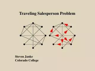
Traveling Salesperson Problem. Steven Janke Colorado College. Traveling Salesperson Problem (TSP). A. B. A B C D. A B C D. C. D. Optimization Problem: Find the least cost tour starting at A, traveling

E N D
Traveling Salesperson Problem Steven Janke Colorado College
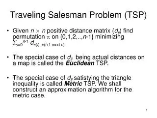
Traveling Salesperson Problem (TSP) A B A B C D A B C D C D Optimization Problem: Find the least cost tour starting at A, traveling through the other three cities exactly once and returning to A. Decision Problem: Is there a TSP tour with cost less than k?
Sir William Hamilton T. P. Kirkman 1805 - 1865 1806 - 1895 In 1856, he published sufficient conditions for a polyhedral graph to have a Hamiltonian circuit. • Discovered quaternions in 1843 • Invented Icosian Game in 1857 • Hamiltonian Circuits
Twentieth Century History • 1931-32 Merrill Flood, A.W.Tucker, Hassler Whitney (Princeton) pose the Traveling Salesperson Problem. • 1947 George B. Dantzig designs simplex method for linear programming. • 1954 Connection with the Assignment Problem established. • 1962 Dynamic programming formalized. • 1972 Karp proved TSP is NP-complete. • 1985 – 2008 Techniques leading to solving a 85,000-city problem
TSP Applications: • School Bus routing. • Robotic welding in the car industry. • Printed circuit board drilling and laser cutting of integrated circuits. • Genome sequencing. Finding most likely ordering of markers. • Job processing: Chemical plants – cost of setup to produce chemicals.
Mathais Herb ‘n Farm Cutler Hall Slocum El Pomar Packard Admissions Office Campus Tour Colorado College
Versions of the TSP: • Complete or Incomplete graph. • Symmetric vs. Asymmetric cost matrix. • Euclidean (Triangle inequality holds.) • Upper Triangular cost matrix. • Circulant cost matrix. • Bipartite graph.
A A B C D B A B C D C D Traveling Salesperson Problem: Find the least cost tour starting at A, traveling through the other three cities exactly once and returning to A.
Generating Permutations: Recursion: A < BCD B < ACD C < ABD D < ABC BDC ADC ADB ACB CBD CAD BAD BAC CDB CDA BDA BCA DBC DAC DAB CAB DCB DCA DBA CBA Single exchange: ABCD CABD DCBA DBAC BACD ACBD DCAB DBCA BCAD ACDB DACB BDCA BCDA CADB ADCB BDAC CBDA CDAB ADBC BADC CBAD CDBA DABC ABDC
Naïve Algorithm 1. List all tours and their costs: A BCD A = 18 A BDC A = 19 A CBD A = 15 A CDB A = 15 A DBC A = 24 A DCB A = 19 2. Find a tour with minimum cost: A CBD A = 15 (one optimal tour)
Timing results for Naïve Algorithm: Cities Seconds Tours Sec/Tour Estimate for 17 cities: 34.9 days (2.09 x 10¹³ tours)
Complexity: • If there are n-1 cities (other than the home city A), then there are (n-1)! possible tours. • The naïve algorithm takes at least (n-1)! steps. • A random algorithm could possibly find an optimal tour in (n-1) steps. • Is there a deterministic algorithm that can find an optimal tour in a polynomial number of steps?
Theorem: (Karp, 1972) TSP is NP-Complete. (That is, every other hard problem is reducible to TSP.) Open problem:Is there a polynomial time algorithm for TSP? If not, can you prove it? (In technical terms, does P = NP?) Solving the open problem earns you $1,000,000 from the Clay Mathematics Institute.
Approaches to the TSP: • Constant TSP: Analyze the cost matrix. • Linear Programming • Euclidean TSP: Probabilistic analysis. • Approximation algorithms • Search techniques • Branch and Bound • Dynamic Programming • Genetic Algorithm • Ant Colony
A Constant TSP B A B C D A B C D C D A BCD A = 22 A CBD A = 22 A DBC A = 22 A BDC A = 22 A CDB A = 22 A DCB A = 22
Theorem: (Constant TSP) • The only cost matrices that give the same cost for all TSP tours are those with entries that satisfy: • cij = ai + bj • Sketch of Proof: • The set C of matrices with constant cost form a linear subspace. • The dimension of C is 2n-1. • The matrices with either a single row of ones or a single column of ones belong to C and any set of 2n-1 of them are linearly independent.
Constant TSP: a b c
x2 Linear Program x1+ x2 = 5.8 Feasible region Minimize: x1+ x2 Subject to: 2x1 + x2 >= 5 x1 + 2x2 >= 6 x1 >= 0 x2 >= 0 x1 x1+ x2 = 1 x1+ x2 = 3.67
The TSP Polytope: • Let x = (xij ) be a vector with an entry 1 indicating that edge ij is included. Entry 0 indicates the edge is excluded. Hence the vector has length equal to the number of edges. • Let xtbe the vector corresponding to the tour t. Polytope P= convex hull of {xt | t is a tour} Interestingly, dim P = |E| - |V| = n(n-3)/2 (Where E is the set of edges and V is the set of vertices.)
Linear Programming formulation of the TSP: Relaxation of the Linear Program: Additional contraints:
Euclidean TSP: The triangle inequality holds for the distance matrix. For any three cities A, B, C, AB + BC >= AC (Note that the distance measure could be something other than the Euclidean distance.) For the Euclidean TSP, the tour does not cross itself. The Euclidean TSP is still NP-Complete, but there are approximation algorithms.
Edge Crossings in Geometric TSP A B e D C Ae + eB >= AB and Ce + eD >= CD AD + CB >= AB + CD
Minimum Spanning Tree: Pick next smallest edge connected to partial tree but not forming a cycle. D 11 C 6 9 E 7 2 4 7 10 9 A 5 B
Minimum Spanning Tree Algorithm: D 11 C 6 9 E 7 2 4 7 10 9 A 5 B To form a TSP tour, trace the minimum spanning tree twice using short cuts if possible. This gives A-E-B-C-D-A. The cost of this tour is 31. The spanning tree has cost 19.
Euclidean Approximation Guarantee: • Let OPT = cost of optimal TSP tour. MST = cost of minimum spanning tree. RMT = cost of route derived from minimum spanning tree. • The optimal TSP tour minus the last edge is a minimum spanning tree, so MST < OPT. • Then RMT <= 2*MST <= 2*OPT • With a little more care the shortcuts can be optimized to give: RMT <= 1.5*OPT • Recently an algorithm scheme was discovered that gives RMT <= (1+e)*OPT for arbitrary e > 0
Approximations for the General TSP: Can an approximation algorithm find a tour that is, say, within 110% of the optimal route? For an approximation algorithm A and TSP instance I, let A(I) be the cost of the tour it generates and let OPT(I) be the optimal cost. Bottom line: No polynomial time algorithm A can guarantee that for all instances I of TSP, A(I) < r OPT(I) for any constant r, unless P=NP. Nevertheless, there are “rules” (called heuristics) that help find good, if not optimal, TSP tours: • Nearest Neighbor • Dissection • Nearest Insertion • Tour Improvement
A Search Tree B C D C D B D B C Little work required. D C D B C B Total nodes: 1+ (n-1) + (n-1)(n-2) + … + (n-1)! (For 4 cities, there are 10 nodes.)
A B C D C D B C B D C C Branch and Bound techniques possibly reduce the number of nodes visited.
Branch and Bound Technique Add A to the possible list and assign arbitrary cost. While the possible list is not empty do: - Select node with smallest estimated cost and remove from list. - Generate children of selected node and add to list. - If children complete a tour, update optimal tour, otherwise estimate cost of completed tour using this child. - If estimated cost is greater than current optimal, remove node from list. Estimate must be a lower bound on the cost and is called the bounding function. Technique depends on how accurate estimate is.
A Possible Bounding Function B(i) : Each node i in the search tree represents a partial tour. Those cities not in the partial tour form a set of “remaining” cities. C1 = cost of partial tour. C2 = sum of the minimum edges into each remaining city. B(i) = C1 + C2 B(i) <= Cost of any tour containing the partial route.
Mathais Shortest Campus Tour: 1281 seconds Herb ‘n Farm Tutt Library Cutler Slocum El Pomar Armstrong Elapsed time: 1.05 seconds Total nodes visited: 710,050
Timing Results for Branch and Bound Algorithm (Average of 3 Instances.) Visited Total Cities Time (Sec) Nodes Nodes 17 City Admission Tour: 1.05 seconds (710,050 nodes visited out of 2x10¹³)
Ant Colony Optimization • Ants find shortest path to food. • They deposit pheromone on trail. • Trails with most pheromone get most ants. • Basic searching behavior has random character.
Ant Colony Optimization Algorithm for TSP: Place some ants at each city and iterate the following: 1. While at city i, an ant calculates a= c / d where c is the amount of pheromone and d is the distance between i and j. 2. Each ant selects a city not already visited with probabilities proportional to the a . 3. After all ants have built a tour, evaporate some fraction of the existing pheromone. 4. Each ant deposits an amount of pheromone inversely proportional to the length of their tour. r s ij ij ij ij ij ij
Mathais Ant Campus Tour: 1291 seconds Herb ‘n Farm Tutt Library Cutler Slocum El Pomar Armstrong Elapsed time: 1.6 seconds Ant Tours: 34,000
Line drawings with TSP routes: (Robert Bosch and Craig Kaplan)
References: • The Traveling Salesman Problem (1985) • - Lawler, Lenstra, Rinnoooy Kan, Shmoys • The Traveling Salesman Problem and its Variations (2002) • - Gutin, Punnen • The Traveling Salesman Problem: A Computational Study (2006) • - Applegate, Bixby, Chvatal, Cook
Dynamic Programming Algorithm: A – BCD EFG – A A – BCD EGF – A A – BCD FGE – A A – BCD FEG – A A – BCD GFE – A A – BCD GEF – A A – CBD FEG – A FEG Optimal g(i, S) = shortest path from i through vertices in S ending at A. g(i, S) = min { c+ g(j, S - {j}) } Optimal tour = g(A, {all vertices}-A) Steps: n2 x 2n i,j j in S