kNN, LVQ, SOM
480 likes | 741 Vues
kNN, LVQ, SOM. Instance Based Learning K-Nearest Neighbor Algorithm (LVQ) Learning Vector Quantization (SOM) Self Organizing Maps. Instance based learning. Approximating real valued or discrete-valued target functions

kNN, LVQ, SOM
E N D
Presentation Transcript
Instance Based Learning • K-Nearest Neighbor Algorithm • (LVQ) Learning Vector Quantization • (SOM) Self Organizing Maps
Instance based learning • Approximating real valued or discrete-valued target functions • Learning in this algorithm consists of storing the presented training data • When a new query instance is encountered, a set of similar related instances is retrieved from memory and used to classify the new query instance
Construct only local approximation to the target function that applies in the neighborhood of the new query instance • Never construct an approximation designed to perform well over the entire instance space • Instance-based methods can use vector or symbolic representation • Appropriate definition of „neighboring“ instances
Disadvantage of instance-based methods is that the costs of classifying new instances can be high • Nearly all computation takes place at classification time rather than learning time
K-Nearest Neighbor algorithm • Most basic instance-based method • Data are represented in a vector space • Supervised learning
In nearest-neighbor learning the target function may be either discrete-valued or real valued • Learning a discrete valued function • , V is the finite set {v1,......,vn} • For discrete-valued, the k-NN returns the most common value among the k training examples nearest toxq.
Training algorithm • For each training example <x,f(x)> add the example to the list • Classification algorithm • Given a query instance xq to be classified • Let x1,..,xk k instances which are nearest to xq • Where (a,b)=1 if a=b, else (a,b)= 0 (Kronecker function)
Definition of Voronoi diagram • the decision surface induced by 1-NN for a typical set of training examples. . _ _ _ . _ . + . + . _ + xq . _ +
kNN rule leeds to partition of the space into cells (Vornoi cells) enclosing the training points labelled as belonging to the same class • The decision boundary in a Vornoi tessellation of the feature space resembles the surface of a crystall
1-Nearest Neighbor query point qf nearest neighbor qi
3-Nearest Neighbors query point qf 3 nearest neighbors 2x,1o
7-Nearest Neighbors query point qf 7 nearest neighbors 3x,4o
How to determine the good value for k? • Determined experimentally • Start with k=1 and use a test set to validate the error rate of the classifier • Repeat with k=k+2 • Choose the value of k for which the error rate is minimum • Note: k should be odd number to avoid ties
Continous-valued target functions • kNN approximating continous-valued target functions • Calculate the mean value of the k nearest training examples rather than calculate their most common value
Distance Weighted • Refinement to kNN is to weight the contribution of each k neighbor according to the distance to the query point xq • Greater weight to closer neighbors • For discrete target functions
Distance Weighted • For real valued functions
Curse of Dimensionality • Imagine instances described by 20 features (attributes) but only 3 are relevant to target function • Curse of dimensionality: nearest neighbor is easily misled when instance space is high-dimensional • Dominated by large number of irrelevant features Possible solutions • Stretch j-th axis by weight zj, where z1,…,zn chosen to minimize prediction error (weight different features differently) • Use cross-validation to automatically choose weights z1,…,zn • Note setting zj to zero eliminates this dimension alltogether (feature subset selection) • PCA
When to Consider Nearest Neighbors • Instances map to points in Rd • Less than 20 features (attributes) per instance, typically normalized • Lots of training data Advantages: • Training is very fast • Learn complex target functions • Do not loose information Disadvantages: • Slow at query time • Presorting and indexing training samples into search trees reduces time • Easily fooled by irrelevant features (attributes)
LVQ(Learning Vector Quantization) • A nearest neighbor method, because the smallest distance of the unknown vector from a set of reference vectors is sought • However not all examples are stored as in kNN, but a a fixed number of reference vectors for each class v (for discrete function f) {v1,......,vn} • The value of the reference vectors is optimized during learning process
The supervised learning • rewards correct classification • puished incorrect classification • 0 < (t) < 1 is a monotonically decreasing scalar function
LVQ Learning (Supervised) Initialization of reference vectors m;t=0; do { chose xi from the dataset mc nearest reference vector according to d2 if classified correctly, the class v of mc is equal to class of v of xi if classified incorrectly, the class v of mc is different to class of v of xi t++; } until number of iterations tmax_iterations
After learning the space Rd is partitioned by a Vornoi tessalation corresponding to mi • The exist extension to the basic LVQ, called LVQ2, LVQ3
LVQ Classification • Given a query instance xq to be classified • Let xanswerbe the reference vector which is nearest to xq, determine the corresponding vanswer
Kohonen Self Organizing Maps • Unsupervised learning • Labeling, supervised • Perform a topologically ordered mapping from high dimensional space onto two-dimensional space • The centroids (units) are arranged in a layer (two dimensional space), units physically near each other in a two-dimensional space respond to similar input
0 < (t) < 1 is a monotonically decreasing scalar function • NE(t) is a neighborhood function is decreasing with time t • The topology of the map is defined by NE(t) • The dimension of the map is smaller (equal) then the dimension of the data space • Usually the dimension of a map is two • For tow dimensional map the number of the centroids should have a integer valued square root • a good value to start is around 102 centroids
SOM Learning (Unsupervised) Initialization of center vectors m;t=0; do { chose xi from the dataset mc nearest reference vector according to d2 For all mrnear mc on the map t++; } until number of iterations tmax_iterations
Supervised labeling • The network can be labeled in two ways • (A) For each known class represented by a vector the closest centroid is searched and labeled accordingly • (B) For every centroid is is tested to which known class represented by a vector it is closest
Example of labeling of 10 classes, 0,..,9 • 10*10 centroids • 2-dim map
Animal example
Ordering process of 2 dim datarandom 2 dim points 2-dim map 1-dim map
Instance Based Learning • K-Nearest Neighbor Algorithm • (LVQ) Learning Vector Quantization • (SOM) Self Organizing Maps
Bayes Classification • Naive Bayes