Lecture 6: Query Processing; Hurry up!
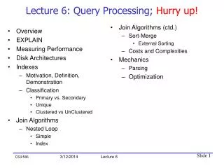
Lecture 6: Query Processing; Hurry up!. Join Algorithms (ctd.) Sort-Merge External Sorting Costs and Complexities Mechanics Parsing Optimization. Overview EXPLAIN Measuring Performance Disk Architectures Indexes Motivation, Definition, Demonstration Classification

Lecture 6: Query Processing; Hurry up!
E N D
Presentation Transcript
Lecture 6: Query Processing; Hurry up! • Join Algorithms (ctd.) • Sort-Merge • External Sorting • Costs and Complexities • Mechanics • Parsing • Optimization • Overview • EXPLAIN • Measuring Performance • Disk Architectures • Indexes • Motivation, Definition, Demonstration • Classification • Primary vs. Secondary • Unique • Clustered vs UnClustered • Join Algorithms • Nested Loop • Simple • Index CS3/586 3/12/2014 Lecture 6
Learning objectives LO6.1: Use SQL to declare indexes LO6.2: Determine the I/O cost of finding record(s) using a B+ tree LO6.3: Given a join query, calculate the cost using each join algorithm: Nested loops, Index Nested Loops, Sort-Merge LO6.4: Parse a query LO6.5: Use VP to answer questions about optimization
Web Form Applic. Front end SQL interface Today we will start from the bottom SQL Security Parser Catalog Relational Algebra(RA) Optimizer Operator algorithms Executable Plan (RA+Algorithms) 3 Concurrency Plan Executor Crash Recovery 2 indexes Files, Indexes & Access Methods how a disk works 1 Database, Indexes
Measuring Query Speed • Our goal this week is to figure out how to execute a query fast. • But the time a query takes to execute is hard to measure or predict. • Depends on environment • Simpler, easier to measure and predict: Number of disk I/Os. • Good: Very roughly proportional to execution time • Bad: Does not take into account CPU time or type of I/O • Therefore: we will use number of disk I/Os to measure the time it takes a query to execute. • Like looking under the lamppost.
Components of a Disk * Spindle Disk head Tracks • platters are always spinning (say, 7200rpm). • one head reads/writes at any one time. • to read a record: • position arm (seek) • engage head • wait for data to spin by • read (transfer data) Sector Platters Arm movement Arm assembly
More terminology Spindle Disk head Tracks • Each track is made up of fixed size sectors. • Page size is a multiple ofsector size. • A platter typically has data on both surfaces. • All the tracks that you can reach from one position of the arm is called a cylinder(imaginary!). Sector Platters Arm movement Arm assembly
Cost of Accessing Data on Disk • Time to access (read/write) a disk block: • seek time (moving arms to position disk head on track) • rotational delay (waiting for block to rotate under head) • Half a rotation, on average • transfer time (actually moving data to/from disk surface) • Key to lower I/O cost: reduce seek/rotation delays!(you have to wait for the transfer time, no matter what) • The text measures the cost of a query by the NUMBER of page I/Os, implying that all I/Os have the same cost, and that CPU time is free. This is a common simplification. • Real DMBSs (in the optimizer) would consider sequential vs. random disk reads – because sequential reads are much faster – and would count CPU time.
Typical Disk Drive Statistics (2009)* Sector size: 512 bytes Seek time Average 4-10 ms Track to track .6-1.0 ms Average Rotational Delay - 3 to 5 ms (rotational speed 10,000 RPM to 5,400RPM) Transfer Time - Sustained data rate 0.3- 0.1 msec per 8K page, or 25-75 Meg/second Density 12-18GB/in2 Rule of Thumb: 100 I-Os/second/page
How far away is the data? From http://research.microsoft.com/~gray/papers/AlphaSortSigmod.doc
Block, page and record sizes • Block – According to text, smallest unit of I/O. • Page – often used in place of block. • My notation is: • Page is smallest I/O for operating system • Block is smallest I/O for an application • Block is integral number of units • “typical” record size: commonly hundreds, sometimes thousands of bytes • Unlike the toy records in textbooks • “typical” page size 4K, 8K
What Block Size is Faster?* • At times you can choose a block size for an application. How? • In some OS's, e.g., IBM's, you can enforce a block size • Or you can perform several reads at once, imitating a large block size. This is called asynchronous readahead. • This is like: should I buy one bottle or a case? • What application will run faster with a large block size? • Goal is for the disk to overlap reads with the CPU's processing of records. Potentially running twice as fast. • What application will run faster with a small block size? • Goal is not to waste memory or read time.
Time for some Magic • You are in charge of a production DBMS for the FEC. • Production: an enterprise depends on the DBMS for its existence. • Customers will ask queries like “find donations from 97223”. You must ensure a reasonable response time. • If the queries run forever, customers will be unhappy and you will be DM. • The DBMS will grind to a halt. Customers will complain to congress, you will be out of a job. • Wouldn't it be nice to know what plan the optimizer will choose, and how long that plan will take to execute? • Rub the magic lantern…
Postgres’ EXPLAIN • Output for EXPLAIN SELECT * FROM indiv WHERE zip = ‘97223’; Seq Scan on indiv (cost=0.00.. 109495.94 rows=221 width=166) Filter:(zip = ‘97223’::bpchar) • These values are estimates from sampling. • Most DBMS's provide this facility. • Also useful when a query runs longer than expected. • If you are online, try it. *Actually this includes CPU costs but we will call it I/O costs to simplify Sequential Scan I/Os to get first row I/Os to get last row* Rows retrieved Average Row Width
You are now DM • More than 100K I/Os! • Response time is 1,000 seconds, or 17 minutes. • Unacceptable! Customers will complain! • Is there a faster way than Seq Scan? • You must do something or you are out of a job!!!
To the Rescue: Index • AnIndex is a data structure thatspeeds up access to records based on some search key field(s). • Indexes are not part of the SQL standard • Because of physical data independence • Typical SQL command to create an index: CREATEINDEX indexname ON tablename (searchkeyname[s]); • For example CREATE INDEX indiv_zip_idx ON indiv(zip); Nota Bene • “Search key” is not the same as a keyfor the table. Attributes in a “search key” need not be unique.
Index Demonstration: Input, Output EXPLAIN SELECT * FROM indiv WHERE zip='97223'; Seq Scan on indiv (cost=0.00..109495.94 rows=221 width=166) Filter: (zip = '97223'::bpchar) CREATE INDEX indiv_zip_idx ON indiv(zip); EXPLAIN SELECT * FROM indiv WHERE zip='97223'; Bitmap Heap Scan on indiv (cost=6.06..861.32 rows=221 width=166) Recheck Cond: (zip = '97223'::bpchar) -> Bitmap Index Scan on indiv_zip_idx (cost=0.00..6.01 rows=221 width=0) Index Cond: (zip = '97223'::bpchar) • With an index, the I/Os went from 109,495 to 861! • That’s 17 minutes to 9 seconds!
LO6.1: Practice with indexes* • When you declare a primary key, most modern DBMSs (including Postgres) create a clustered (sorted) index on the primary key attribute (s). • Give the SQL for creating all possible single-attribute indexes on the table Emp(ssn PRIMARY KEY, name) • What are the search keys of each index?
Data Entries* • Before we learn about how indexes are built, we must understand the concept of data entries. • Given a search key value, the index produces a data entry, which produces the data record in one I/O. • Other real-life indexes will help motivate this concept. • Each of the following indexes speeds up data retrieval. What is the search key, data entry, and data record for each one? Search Key Data Entry Data Record Library Catalog Google Mapquest
Essentially all DBMS Indexes are B+ Trees • Oracle, SQLServer and DB2 support only B+Tree indexes. Postgres supports hash indexes but does not recommend using them. • B+ tree indexes support range searches (WHERE const < attribute)and equality searches (WHERE const = attribute). • The next page contains a sample B+ tree index. Think of it as an index on the first two digits of zip code. • 28* is a data entry that points to the donations from zip codes that start with 28. • Above the data entries are index entries that help find the correct data entry.
Root 17 Entries <= 17 Entries > 17 27 5 13 30 39* 2* 3* 5* 7* 8* 22* 24* 27* 29* 38* 33* 34* 14* 16* Example B+ Tree Note how data entries in leaf level are sorted • Find 29*? 28*? All > 15* and < 30* • Insert/delete: Find data entry in leaf, then change it. Need to adjust parent sometimes. • And change sometimes bubbles up the tree • This keeps the tree balanced: each data retrieval takes the same number of I/Os. • Each page is always at least half full.
LO6.2: I/O Cost in a B+ Tree* Root 17 27 5 13 30 39* 2* 3* 5* 7* 8* 22* 24* 27* 29* 38* 33* 34* 14* 16* How many I/Os are required to retrieve data records with search key values x, 13 < x < 27? Assume x is a unique key. How many I/Os are required to retrieve data records with search key values x, 3 < x < 15? Assume x is a unique key.
index entry P K P K P P K m 0 1 2 1 m 2 B+ Tree Indexes Non-leaf Pages Leaf Pages (Sorted by search key) • Leaf pages containdata entries, and are chained (prev & next) • Non-leaf pages have index entries; only used to direct searches:
Don’t get carried away!* • Now I don’t want you to run out and index every attribute and set of attributes in all your tables! • If you define an index, you will incur three costs • Space to store the index • Updates to the search key will be slower – why? • The optimizer will take longer to choose the best plan because it has more plans to choose from. • We will see that sometimes it is better not to use an index • There is one advantage to having an index • Some queries run faster (better be sure about this).
Index Classification • Primary vs. secondary: If the index’s search key contains the relation’s primary key, then the index is called a primary index, otherwise a secondary index. • The index created by the DBMS for the primary key is usually called the primary index. • Unique index: Search key contains a candidate key, i.e. no duplicate values of the search key.
Index entries UNCLUSTERED CLUSTERED direct search for data entries Data entries Data entries (Index File) (Data file) Data Records Data Records Clustered vs. Unclustered indexes • If the order of the data records is the same as, or `close to’, the order of the search key, then the index is called clustered.
Comments on Clustered Indexes • If you are retrieving only one record, any index will do. • Retrieve one record in each index and count the I/Os. • Assume the height of the index entry tree is 2. • If you are retrieving many records with the same search key value, a clustered index is almost always faster. • Retrieve 10 records from each index and count the I/Os. • Clustered: • Unclustered: • Lest you get carried away: a table can have only one clustered index. Why? • DBMSs make their primary indexes clustered. • PS: DB2, Postgres and MySQL construct clustered indexes as we have described on the previous slide. Oracle and SQLServer put the data records in place of the data entries.
Where Are We? • We've now learned two ways to perform a 1-table SELECT query: Sequential Scan and Index Scan. • EXPLAIN tells you which plan/algorithm the optimizer will choose; which one it thinks is the fastest. • Now we study possible plans/algorithms for multi-table join SELECT queries.
Join Algorithms: Motivation (apocryphal) • When I was young I was asked to help with a charity art auction. At the start I got a big stack of bidder cards with bidder IDs and bidder information. • At the end I got a much bigger stack of bought cards, each one containing a bidder ID and the cost of a painting that a bidder bought. • Suddenly there was a long line of bidders who wanted to go home. For each bidder, I had to give the cashier the bidder’s card with the bidder’s matching bought cards. • What would you do if you were in this situation?
Computer Science Algorithms • Answers to the previous question will be investigated on the following pages. They fall into three categories, the three basic algorithms of computer science: iteration, sorting and hashing. • Nested Loop Join (iteration) comes in two versions: • Simple Nested Loop • Index Nested Loop • Sort Merge Join • Hash Join (Will not be covered in this course)
Join Algorithms – an Introduction • The text discusses algorithms for every relational operator. We study only join algorithms since join is so expensive. • L⋈R is very common! • Notation: M pages in L, pL rows per page, N pages in R, pR rows per page. • In our examples, L is indiv and R is comm. • Our algorithms work for any equijoins.
A simple join SELECT * FROM indiv L, comm R WHERE L.commid=R.commid Review how to compute this join by hand, with the cl versions of the tables. M = 23,224 pages in L, pL = 39 rows per page, N = 414 pages in R, pR = 24 rows per page. These (estimated) statistics are stored in the system catalog. In PostgreSQL, retrieve number of pages with the function SELECT pg_relation_size('tablename')/8192; Retrieve rows per page using SELECTCOUNT(*)/(pages in L or R) FROM L or R;
The simplest algorithm: Nested Loops Join on commid in L and commid in R foreachrow lin L do foreachrow rin R do if rcommid == lcommid then add <r, s> to result • For each row in the outer table L, we scan the entire inner table R, row by row. • Cost: M + (pL * M) * N = 23,224 + (39*23,224)*414 I/Os = 374,997,928 I/Os 3,749,979 seconds 43 days Assuming approximately 100 I/Os per second (86,400 secs/day)
Nested Loops Join Table L on disk Table R on disk Memory Buffers: 2 ... 12 … 6 ... ... 2 … 13 … 12 … 27 1 … 5 … 27 … … 1 … 5
Nested Loops Join Table L on disk Table R on disk Memory Buffers: 2 ... 12 … 6 ... 2 ... 12 … 6 ... ... 2 … 13 ... 2 … 13 … 12 … 27 1 … 5 … 27 … … 1 … 5 Query Answer 2 … … 2
Nested Loops Join Table L on disk Table R on disk Memory Buffers: 2 ... 12 … 6 ... 2 ... 12 … 6 ... ... 2 … 13 ... 2 … 13 … 12 … 27 1 … 5 … 27 … No match: Discard! … 1 … 5 Query Answer 2 … … 2
Nested Loops Join Table L on disk Table R on disk Memory Buffers: 2 ... 12 … 6 ... 2 ... 12 … 6 ... ... 2 … 13 … 12 … 27 … 12 … 27 1 … 5 … 27 … No match: Discard! … 1 … 5 Query Answer 2 … … 2
Nested Loops Join Table L on disk Table R on disk Memory Buffers: 2 ... 12 … 6 ... 2 ... 12 … 6 ... ... 2 … 13 … 12 … 27 … 12 … 27 1 … 5 … 27 … No match: Discard! … 1 … 5 Query Answer 2 … … 2
Nested Loops Join Table L on disk Table R on disk Memory Buffers: 2 ... 12 … 6 ... 2 ... 12 … 6 ... ... 2 … 13 … 1 … 5 … 12 … 27 1 … 5 … 27 … No match: Discard! … 1 … 5 Query Answer 2 … … 2
Nested Loops Join Table L on disk Table R on disk Memory Buffers: 2 ... 12 … 6 ... 2 ... 12 … 6 ... ... 2 … 13 … 1 … 5 … 12 … 27 1 … 5 … 27 … No match: Discard! … 1 … 5 Query Answer 2 … … 2
Nested Loops Join Table L on disk Table R on disk Memory Buffers: 2 ... 12 … 6 ... 2 ... 12 … 6 ... ... 2 … 13 ... 2 … 13 … 12 … 27 1 … 5 … 27 … No match: Discard! … 1 … 5 Query Answer 2 … … 2
Nested Loops Join Table L on disk Table R on disk Memory Buffers: 2 ... 12 … 6 ... 2 ... 12 … 6 ... ... 2 … 13 ... 2 … 13 … 12 … 27 1 … 5 … 27 … No match: Discard! … 1 … 5 Query Answer 2 … … 2
Nested Loops Join Table L on disk Table R on disk Memory Buffers: 2 ... 12 … 6 ... 2 ... 12 … 6 ... ... 2 … 13 … 12 … 27 … 12 … 27 1 … 5 … 27 … Match! … 1 … 5 And so forth … Query Answer 2 … … 2 12 … … 12
Index Nested Loops Join IF THERE IS AN INDEX ON r.commid foreach row l in L do use the index to find all rowsr in R where lcommid = rcommid for all such r: add <l, r> to result Cost: M + ( (M*pL) * cost of finding matching R rows) = 23224 + ((23224*39)*3) = 2,740,432 I/Os 27,404 secs 8 hours Cost of finding the rows in R using the index on commid – much cheaper than scanning all of comm!
78 72 68 55 54 54 40 36 23 21 20 18 9 7 92 88 66 51 43 29 External Sorting • Many relational operator algorithms require sorting a table • Often the table won’t fit in memory • How do we sort a dataset that won’t fit in memory? • Answer: External Sort-Merge algorithm • First pass: Read and write a memoryfull of (sorted) runs at a time. • Second and later passes: Merge runs to make longer runs • Here’s a picture of merging two runs: The merged output is a longer run, on disk Runs on disk Merging the runs in memory
External Sorting – Cost • Number of passes depends on how many pages of memory are devoted to sorting • Can sort M pages of data using B pages of memory in 2 passes if sqrt(M) <= B • Can sort big files M with not much memory B • If page size is 4K: • Can sort 4Gig of data in 4Meg of memory • Can sort 256Gig of data in 32Meg of memory • Each pass is a read and a write, so if sqrt(M) <= B then sort costs (M+M)+(M+M) so can be done in 4*M I/Os • So it’s reasonable to assume that sorting M pages costs 4*M.
Sort-Merge Join • This join algorithm is the one many people think of when asked how they would join two tables. It is also the simplest to visualize. It involves three steps. • Sort L on lcommid • Sort R on rcommid • Merge the sorted L and R on lcommid and rcommid. • We’ve covered the algorithm and cost of steps 1 and 2 on the previous pages
The Merge Step • What is the algorithm for step 3, the merge? • Advance scan of L until current L-row’s lcommid >= current R row’s rcommid, then advance scan of R until current R-row’s rcommid >= current R row’s lcommid ; do this until current R row’s lcommid = current R row’s rcommid. • At this point, all R rows with same lcommid and all R rows with same rcommidmatch; output <l, r> for all pairs of such rows. • Then resume scanning L and R. • What is the cost of the merge step? • Normally, M+N • What if there are many duplicate values of lcommid and rcommid? • What if all values of lcommid are the same and equal to all values of rcommid? • Then L ⋈ R = L R and the cost of the merge step is L * R. • BUT, almost every real life join is a foreign key join. One of the joining attributes is a key, so the duplicate value problem does not occur.
Cost of Sort-Merge Join • Assuming that sorting can be done in two passes and that the join is a foreign key join • Cost: (cost to sort L) + (cost to sort R) + (cost of merge) = 4M + 4N + (M+N) = 5(M+N) • For our running example the cost is: 5*(M+N) = 5*(23224+414) = 118,190 I/Os 1,181 seconds 20 minutes • In reality the cost is much less because of optimizations, indexes, and the use of hash join • Cf. CS587/410
Costs for Join Algorithms *For homework and exercises you may assume this is 3 times the number of rows retrieved
LO6.3: Costs of Join Algorithms* • Consider this join query: SELECT * FROM pas L, comm R WHERE L.commid = R.commid; • Calculate the cost (in time) of a nested loop, index nested loop and sort-merge join.