Download
1 / 57
590 likes | 800 Vues
ESTIMATING THE MASSES OF ELEMENTARY PARTICLES. Rajan Gupta Los Alamos National Laboratory. A FASCINATING STORY OF THE DISCOVERY AND IDENTIFICATION OF ELEMENTARY PARTICLES, AND THE SUBSEQUENT DETERMINATION OF THEIR MASSES. Elementary Particles.

E N D
ESTIMATING THE MASSES OF ELEMENTARY PARTICLES Rajan Gupta Los Alamos National Laboratory
A FASCINATING STORY OF THE DISCOVERY AND IDENTIFICATION OF ELEMENTARY PARTICLES, AND THE SUBSEQUENT DETERMINATION OF THEIR MASSES.
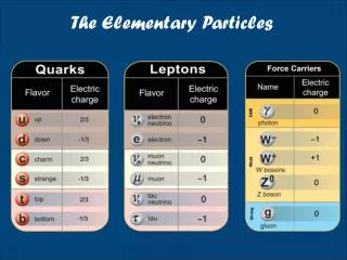
Elementary Particles With our current understanding, the world of elementary particles is first encountered at the level of atoms (10-10 m) • Electrons • Nucleus nucleons (protons, neutrons) quarks and gluons
Standard Model L = L(QCD) + L (SU(2)L U(1)Y ) + L (Higgs) + L (Y) L(QCD) =- 1/4 Ga Ga +Q ( i + gaAa )Q L (SU(2)L U(1)Y ) = -1/4 Wa Wa -1/4 B B + L (g2aWa + g1Y B ) L +R (g2aWa + g1Y B ) R + L(i ) L L (Y) = Q MqQ + L Ml L + Mq/vQHQ +Ml/ v LHL L (Higgs) = (D )†(D ) -(-h2 † + h /4 (†)2 )
Electro- Coulomb, Faraday, Maxwell (1864) magnetism QED Tomonaga, Schwinger, Feynman 1949 Weak Fermi 1934 (Fermi Theory) Marshak & Sudarshan, Feynman & Gell-mann 1958 (V-A) Electro- Glashow, Salam, Weinberg 1969; weak ‘t Hooft & Veltman 1972 (renormalizable) QCD Gellmann, Zweig 1963 (quarks) Quarks and gluons (dynamics) 1972 Politzer, Gross & Wilczek(1973 asymptotic freedom) History of the Standard Model
Relativity: Einstein 1905-1915 Quantum Bohr, Born, de Broglie, Heisenberg, Mechanics: Pauli, Schrodinger, 1913-1927 Antimatter: Dirac 1928 Non-abelian Yang & Mills, 1954 Higgs Higgs 1964 KEY IDEAS IN THE THEORY
WHERE ARE THE ELEMENTARY PARTICLES ELECTRONS (e), MUONS (), THEIR NEUTRINOS (e ,), PHOTONS (), ARE THE ONLY ELEMENTARY PARTICLES THAT EXIST COPIOUSLY IN NATURE. ALL OTHERS HAVE TO BE CREATED IN HIGH ENERGY ACCELERATORS AND THEN STUDIED IN COMPLEX DETECTORS
E increases E by E = Fd = qV = qEd Constant B bends beam in a circle of radius = pc/qB S1 B S2 PARTICLE ACCELERATORS Accelerators are based on 2 properties of the electromagnetic force F = q(E + vB) V=Ed E = qV
SLAC (e-, e+) OTHER(e-, e+) MACHINES: CORNELL, DESY, LEP
FERMILAB (p,p) OTHER(p,p) MACHINES: CERN (LHC)
COMPLEX, MULTILAYERED & HUGE PARTICLE DETECTORS CDF in collision hall Inserting the silicon vertex tracker in the 2000 ton central detector. West plug also shown Electronics on beam pipe Curtsey of FNAL & CDF collaboration
E2 = p2c2 + m2c4 & p = mv E = h and p = h/ Pole in the propagator Axial Symmetry relation between currents WHAT IS MASS knowing E & p gives m
Are the particles sufficiently “long-lived” to leave a measurable track Are they electrically charged Do they have well-defined decay channels DETERMINING MASSES PROPERTIES THAT FACILITATE DETECTION
e Tracks in B field e, LEPTONS ARE EASY TO PRODUCE & DETECT
CHARGED LEPTONS Mass Mean life time e+ , e- 0.511 MeV Stable +, - 105.7 MeV 2.197 × 10⁻⁶ sec +, - 1777 MeV 290.6 × 10⁻¹⁵ sec Experiments utilize incident beams of e+, e- and of +, -
e+ , e- J. J. Thompson using cathode tube at Cavendish in 1897. Millikan measured the basic unit of charge in 1909 +, - Neddermeyer and Anderson in cosmic ray experiments in 1937(also Stevenson & Street and Nishina Group) +, - Martin Perl at SLAC in 1976 HISTORY OF CHARGED LEPTONS
FORCE CARRIERS Mass Width |Mean life time (photon)0 Stable g (gluons)0 Confined W+, W- 80.42 GeV 2.12 GeV (3.1 × 10⁻²⁵ sec ) Z 91.19 GeV 2.50 GeV (2.6 × 10⁻²⁵ sec ) Experiments can create photon beams
Antiquity. Planck introduced “quanta” in 1900. Einstein established particle nature by describing photoelectric effect in 1905. g 3 jet events reported at DESY in 1979; the third jet interpreted as due to a gluon W, Z Discovered at CERN in 1982(Rubbia) HISTORY OF FORCE CARRIERS
q q q q e+ e- e+ e- g Examples of 2-jet and 3-jet events observed in the JADE detector at the PETRA e+ e- collider at 30, 31 GeV in cm (DESY)
Three or more jets signify production of qq and additional particles (gluons within the framework of QCD) that also form jets. The ratio of 3-jet/2-jet (and 4-jet/2-jet, …) cross-sections is consistent with gluon production in QCD The change in these ratios of cross-sections with energy is consistent with QCD JETS GLUONS
States produced as resonances in e+e- Annihilation e+ l, q X ,Z0 e- l, q s = cm energy, GeV s = cm energy, GeV (e+e- hadrons) (e+e- + - ) R = Nci ei2 = Vector boson resonances
l, q l, q Resonance in p+p- Interactions q X g, ,Z0 q
+ - + - W+ W- Z0 Charmonium (J/, ….) Bottomonium (/// , …..) Top RESONANCES PARTICLES LEAD TO THE DISCOVERY/PRODUCTION OF
e+e- hadrons e+e- ,+- CHARMONIUM(cc) SLAC (Richter, 1974) BNL (Ting, 1974) p + Be J/ + anything e+e- Such experiments gave the masses of cc bound states. mc?
BOTTOMONIUM(bb) CLEO at CESR FNAL (1977) p + Be, Cu, Pt + +- + anything e+e- hadrons e+e- ,+- The /// are not resolved in the broad peak
(t t ) too short lived to form onia p+ p- t + t + anything W-b W+b W e W W q q jet b, b jet Artist’s view of top event at CDF
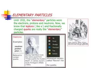
QUARKS quark Name Mass (MS) u up2-4 MeV QCD d down4-6 MeV QCD s strange70-120 MeV QCD c charm 1.15-1.5 GeV b bottom 4.0 - 4.4 GeV t top 168+10 GeV 1963 1974 1977 1995 -7
Quarks are not seen as asymptotic states but confined within hadrons! Experiments provide masses of mesons (, K, , /, , , J/, ,...) and baryons (N, , , , , ...) Decays products are heavier than the quarks due to hadronization! Quarks always dressed by gluons The QCD coupling is large, s1, at hadronic scales. Gluon effects are large (~ 300 MeV ~ QCD) MASSES OF QUARKS How do we measure quark masses?
QCD: Cannot solve it analytically in the low energy region. USE Chiral Lagrangian: Low energy effective theory of , K, mesons. Same symmetries as QCD. Quark masses are parameters. RESORT TO THEORY AND RELATE HADRON MASSES TO QUARKS LATTICE QCD QCD SUM RULES
Parameters of this effective theory include quark masses. Determine these parameters by fitting the observed meson masses and decays to predictions of PT Can extract only ratios of light quark masses (mu/md, md/ms) as theory has an overall unknown scale. CHIRAL PERTURBATION THEORY
(A12) = (m1 + m2) P12 (V12) = (m1 - m2) S12 x (A12) (x,t) J(0,0) (m1 + m2) = x P12(x,t) J(0,0) DEFINITION OF mq in QCD CURRENT CONSERVATION IN QCD Calculate 2-point correlation functions (J is a source for pions)
QCD SUM-RULES (A12) (x,t) (A12) (0,0) = (m1 + m2)2 P12(x,t) P12(0,0) Spectral function OPERATOR PRODUCT EXPANSION + PERTURBATION THEORY
masses of quarks the gauge coupling SOLVE QCD NUMERICALLY Solve for the spectrum of mesons and baryons using Monte Carlo simulations of LATTICE QCD with input values for Tune mquark until masses of all hadrons agree with experimental values.
Generate background gauge configurations {U(x)} distributed with probability given by the QCD action Calculate Feynman quark propagators SF[U] on these background configurations Average correlation functions constructed out of {U(x)} and SF[U] over these configurations (do the functional integral) LATTICE QCD Field theory in Euclidean space
LATTICE QCD QCD (g, mu, md, ms, mc, mb) GAUGE CONFIGURATIONS LATTICE QCD $ QUARKPROPAGATORS Systematic errors Statistical errors
QUARK MASSES(MS) Chiral Perturbation theory mu / md = 0.55(4) 2ms / (mu +md) = 24.4(1.5) LQCD Sum Rules mu (2GeV)2.2-2.7 MeV 2.4-3.8 MeV md (2GeV)4.3-6.9 MeV 4.3-6.9 MeV ms (2GeV)78-100 MeV 83-130 MeV Mc (Mc) 1.2-1.6 GeV 1.25(10) GeV Mb (Mb) 4.3(1) GeV 4.2(1) GeV
Electrically neutral Have only weak interactions Masses very small NEUTRINOSe,e,,,,
time time Neutrino interactions are weak ne ne ne ne + Z W- e- e- e- e- Charged current Neutral current very small!
DECTECTING NEUTRINOS THE INCIDENT NEUTRINO IS INVISIBLE. DETECTORS “SEE” THE CHARGED PRODUCTS
e type event Curtsey: B Blumenfeld, JHU
type event Curtsey: B Blumenfeld, JHU
NEUTRINOS /m Mass e< 3 eV > 7 109 sec/eV < 0.19 MeV > 15.4 sec/eV < 18.2 MeV Experiments utilize incident beams of ee
History of Neutrino Physics • 1914: Chadwick finds decay spectrum to be continuous • 1930: W. Pauli proposed ‘neutron’ as an explanation • 1936: Fermi-Gamow-Teller theory with a “neutrino” • 1956: Cowan and Reines observe einteractions • 1958: V-A theory of weak processes • 1962: Danby et al, observe interactions • 1990: Precisely 3 light neutrinos exist in nature • 2000: DONUT collaboration observes interactions
NEUTRINO MASSES e : End point of the tritium beta decay spectrum n p + e + e : End point of the pion decay spectrum
M from missing energy Beta decay spectrum for molecular tritium