Download
1 / 15
150 likes | 176 Vues
Explore the innovative concept of "map-ematics" merging math and GIS for advanced analytical insights. Discover spatial analysis operations and the evolution of GIS into a powerful problem-solving tool. Delve into the future directions of map analysis and modeling with a focus on quantitative analysis of map variables.

E N D
Future Directions of Map Analysis and Modeling: …where we are headed and how we get there 2013 Arkansas GIS Symposium The State of GIS | September 9th - 13th 2013 “They who don’t know, don’t know they don’t know” Presentation Premise: There is a“map-ematics”that extends traditional math/stat concepts and procedures for thequantitative analysis of map variables(mapped data) This PowerPoint with notes and online links to further reading is posted at www.innovativegis.com/basis/Present/Arkansas_Sep2013/ Presentation byJoseph K. Berry Keck Scholar in Geosciences, Department of Geography, University of Denver Adjunct Faculty in Natural Resources, Warner College of Natural Resources, Colorado State UniversityPrincipal, Berry & Associates // Spatial Information Systems Email: jberry@innovativegis.com— Website: www.innovativegis.com/basis
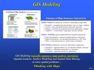
Making a Case for SpatialSTEM (Setting the Stage) The lion’s share of the growth has been GIS’s ever expanding capabilities as a “technical tool” for corralling vast amounts of spatial data and providing near instantaneous access to remote sensing images, GPS navigation, interactive maps, asset management records, geo-queries and awesome displays. However, GIS as an “analytical tool” hasn’t experienced the same meteoric rise— in fact it can be argued that the analytic side of GIS has somewhat stalled… partly because of… …but modern digital “maps are numbers first, pictures later” and we do mathematical and statistical things to map variables that moves GIS from— “WhereisWhat”graphical inventories, to a “Why, So What and What If” problem solving environment— “thinking analytically with maps” (Berry)
Mapping vs. Analyzing (Processing Mapped Data) • …GISis a Technological Tool involving — • Mappingthat creates a spatial representation of an area • Displaythat generates visual renderings of a mapped area • Geo-querythat searches for map locations having a specified classification, condition or characteristic • …and an Analytical Tool involving — • Spatial Mathematics that applies scalar mathematical formulae to account for geometric positioning, scaling, measurement and transformations of mapped data • Spatial Analysis that investigates the contextual relationships within and among mapped data layers • Spatial Statistics that investigates the numerical relationships within and among mapped data layers “Map” “Analyze” Geographic Information Systems (map and analyze) (Descriptive Mapping) (Prescriptive Modeling) Global Positioning System (locate and navigate) Remote Sensing (measure and classify) GPS/GIS/RS (Berry)
A Mathematical Structure for Map Analysis/Modeling GeotechnologyRS – GIS – GPS Technological Tool Analytical Tool Mapping/Geo-Query(Discrete, Spatial Objects) (Continuous, Map Surfaces) Map Analysis/Modeling Geo-registered Analysis Frame Matrix of Numbers Map Stack “Map-ematics” Maps as Data, not Pictures Vector & Raster — Aggregated & Disaggregated Qualitative &Quantitative …organized set of numbers Grid-based Map Analysis Toolbox Spatial Analysis Operations Spatial Statistics Operations Functions GISer’s Perspective: GISer’s Perspective: Local Focal Reclassify andOverlay Distance andNeighbors Surface Modeling Spatial Data Mining Zonal Global Operators Procedures Mathematician’s Perspective: Statistician’s Perspective: Basic GridMath & Map Algebra Advanced GridMath Map Calculus Map Geometry Plane Geometry Connectivity Solid Geometry Connectivity Unique Map Analytics Basic Descriptive Statistics Basic Classification Map Comparison Unique Map Statistics Surface Modeling Advanced Classification Predictive Statistics The SpatialSTEM Framework Traditional math/stat procedures can be extended into geographic space to stimulate those with diverse backgrounds and interests for… “thinking analytically with maps” (Berry)
Spatial Analysis Operations(Geographic Context) GIS as “Technical Tool” (Where is What) vs. “Analytical Tool” (Why, So What and What if) Map Stack Grid Layer Spatial Analysis Spatial Analysisextends the basic set of discrete map features (points, lines and polygons) to map surfaces that represent continuous geographic space as a set of contiguous grid cells (matrix), thereby providing a Mathematical Framework for map analysis and modeling of the Contextual Spatial Relationships within and among grid map layers Mathematical Perspective: Basic GridMath & Map Algebra ( + - * / ) Advanced GridMath (Math, Trig, Logical Functions) Map Calculus (Spatial Derivative, Spatial Integral) Map Geometry (Euclidian Proximity, Effective Proximity, Narrowness) Plane Geometry Connectivity (Optimal Path, Optimal Path Density) Solid Geometry Connectivity (Viewshed, Visual Exposure) Unique Map Analytics (Contiguity, Size/Shape/Integrity, Masking, Profile) Map Analysis Toolbox Unique spatial operations (Berry)
Spatial Analysis Operations(Math Examples) Spatial Derivative Advanced Grid Math —Math, Trig, Logical Functions MapSurface 2500’ …is equivalent to the slope of thetangent plane at a location Map Calculus —Spatial Derivative, Spatial Integral 500’ The derivativeis the instantaneous “rate of change” of a function and is equivalent to the slope of thetangent line at a point Surface Fitted Plane Slope draped over MapSurface Curve SLOPE MapSurfaceFitted FOR MapSurface_slope 65% Spatial Integral Dzxy Elevation 0% ʃ Districts_AverageElevation …summarizes the values on a surface for specified map areas (Total= volume under the surface) Advanced Grid Math Surface Area COMPOSITE Districts WITH MapSurface Average FOR MapSurface_Davg …increases with increasing inclination as a Trig function of the cosine of the slope angle MapSurface_Davg S_Area= Fn(Slope) S_area= cellsize / cos(Dzxy Elevation) Surface Theintegral calculates the area under the curve for any section of a function. Curve (Berry)
Spatial Analysis Operations(Distance Examples) 96.0minutes …farthest away by truck, ATV and hiking Map Geometry —(Euclidian Proximity, Effective Proximity, Narrowness) Plane Geometry Connectivity —(Optimal Path, Optimal Path Density) Solid Geometry Connectivity—(Viewshed, Visual Exposure) HQ(start) Distance Euclidean Proximity Effective Proximity Off Road Relative Barriers On Road 26.5minutes …farthest away by truck Off Road Absolute Barrier On + Off Road Travel-Time Surface Farthest (end) Plane Geometry Connectivity HQ (start) Shortest straight line between two points… …from a point to everywhere… …not necessarily straight lines (movement) Truck = 18.8 min ATV = 14.8 min Hiking = 62.4 min …like a raindrop, the “steepest downhill path” identifies the optimal route (Quickest Path) Solid Geometry Connectivity Rise Visual Exposure Run Tan = Rise/Run • Counts • # Viewers Seen if new tangent exceeds all previous tangents along the line of sight Sums Viewer Weights Splash Highest Weighted Exposure 270/621= 43% of the entire road network is connected Viewshed (Berry)
Spatial Statistics Operations(Numeric Context) GIS as “Technical Tool” (Where is What) vs. “Analytical Tool” (Why, So What and What if) Map Stack Grid Layer Spatial Statistics Spatial Statisticsseeks to map the variation in a data set instead of focusing on a single typical response (central tendency), thereby providing a Statistical Framework for map analysis and modeling of the Numerical Spatial Relationships within and among grid map layers Statistical Perspective: Basic Descriptive Statistics (Min, Max, Median, Mean, StDev, etc.) Basic Classification(Reclassify, Contouring, Normalization) Map Comparison (Joint Coincidence, Statistical Tests) Unique Map Statistics (Roving Window and Regional Summaries) Surface Modeling (Density Analysis, Spatial Interpolation) Advanced Classification (Map Similarity, Maximum Likelihood, Clustering) Predictive Statistics (Map Correlation/Regression, Data Mining Engines) Map Analysis Toolbox Unique spatial operations (Berry)
Spatial Statistics (Linking Data Space with Geographic Space) Roving Window (weighted average) Spatial Distribution Geo-registered Sample Data Spatial Statistics Continuous Map Surface Discrete Sample Map Non-Spatial Statistics Surface Modeling techniques are used to derive a continuous map surface from discrete point data– fits a Surface to the data (maps the variation). Standard Normal Curve Average = 22.6 …lots of NE locations exceed Mean + 1Stdev In Geographic Space, the typical value forms a horizontal plane implying the average is everywhere to form a horizontal plane StDev = 26.2 (48.8) X + 1StDev = 22.6 + 26.2 = 48.8 Histogram In Data Space, a standard normal curve can be fitted to the data to identify the “typical value” (average) X= 22.6 80 0 30 40 50 60 70 10 20 Unusually high values Numeric Distribution +StDev Average (Berry)
Spatial Statistics Operations(Data Mining Examples) Map Clustering: Elevation vs. Slope Scatterplot Cluster 2 “data pair” of map values …as similar as can be WITHIN a cluster …and as different as can be BETWEEN clusters “data pair” plots here in… Data Space Elevation (Feet) Geographic Space Slope draped on Elevation + + Cluster 1 Slope Slope (Percent) Elev X axis = Elevation (0-100 Normalized) Y axis = Slope (0-100 Normalized) Geographic Space Advanced Classification (Clustering) Data Space Map Correlation: Spatially Aggregated Correlation Scalar Value– one value represents the overall non-spatial relationship between the two map surfaces Roving Window r = .432 Aggregated …1 large data table with 25rows x 25 columns = 625 map values for map wide summary Map of the Correlation Entire Map Extent Elevation (Feet) r = …where x = Elevation value and y = Slope value and n = number of value pairs …625 small data tables within 5 cell reach = 81map values for localized summary Slope (Percent) Localized Correlation Map Variable– continuous quantitative surface represents the localized spatial relationship between the two map surfaces Predictive Statistics (Correlation) (Berry)
Grid-based Map Data (geo-registered matrix of map values) 2.50 Latitude/Longitude Grid (140mi grid cell size) 90 Analysis Frame (grid “cells”) 300 Coordinate of first grid cell is 900 N 00 E #Rows= 73 #Columns= 144 Conceptual Spreadsheet(73 x 144) The Latitude/Longitude grid forms a continuous surface for geographic referencing where eachgrid cell represents a given portion of the earth’ surface. Lat/Lon …each 2.50grid cell is about 140mi x 140mi 18,735mi The easiest way to conceptualize a grid map is as an Excel spreadsheet with each cell in the table corresponding to a Lat/Lon grid space (location) and each value in a cell representing the characteristic or condition (information) of a mapped variable occurring at that location. …from Lat/Lon “crosshairs to grid cells” that contain map valuesindicating characteristics or conditions at each location …maximum Lat/Lon decimal degree resolution is a four-inch square anywhere in the world …the bottom line is that… All spatial topology is inherent in the grid. (Berry)
Grid-based Map Data (moving Lat/Lon from crosshairs to grid cells) …Spatially Keyed data in the cloud are downloaded and configured to the Analysis Frame defining the Map Stack Lat/Lon serves as a Universal dB Key for joining data tables based on location Spatially Keyed data in the cloud Conceptual Organization RDBMS Organization Spreadsheet 30m Elevation (99 columns x 99 rows) “Where” Wyoming’s Bighorn Mts. Database Keystone Concept Each of the conceptual grid map spreadsheets (matrices) can be converted to interlaced RDBMS formatwith a long string of numbers forming the data field (map layer) and the records (values) identifying the information at each of the individual grid cell locations. Geographic Space Grid Space 2D Matrix 1D Field Database Table Lat/Lon as a Universal Spatial Key Elevation Surface Once a set of mapped data is stamped with its Lat/Lon “Spatial Key,” it can be linked to any other database table with spatially tagged records without the explicit storage of a fully expanded grid layer— all of the spatial relationships are implicit in the relative Lat/Lon positioning. Data Space Each column (field) represents a single map layer with the values in the rows indicating the characteristic or condition at each grid cell location (record) “What” (Berry)
5-step Process to Unlocking Universal Spatial Data Spatially Aware Database (XY, Value) Step 1. User identifies the geographic extent of the analysis window. Step 2. User specifies thecell size of the analysis window. Where(XY) …Lat/Lon coordinates identify earth position of a dB record 3 6 7 0 What(Value) …value indicates characteristic or condition at a location 1 Longitude 8 11 4 4 9 0 15 7 13 7 20 9 Latitude Step 3. Computer determines the Lat/Lon ranges defining each grid cell (cutoffs) and the centroid location. …defines the Analysis Frame 3 2 7 2 1 13 6 12 11 0 10 3 4 16 5 2 6 1 Step 4. Computer determines the appropriate grid cellfor each database record that falls within the analysis frame’s geographic extent based on its Lat/Lon coordinates the repeat for all selected dB records. Step 5. Computer summarizes the values if more than one value “falls” into an individual grid cell-- result is a “Grid Map Layer” for inclusion in a map stack for subsequent map analysis. Analysis Frame (grid map layer) Shish Kebab of numbers …but Lat/Lon grid cells are only square at the equator— so is the entire idea a bust? Hint: spatial resolution is key (Berry)
The Bottom of the Bottom Line Data Providers/GIS Specialistscreate spatially consistent mapped data and maintain GIS databases; very knowledgeable in GPS, RS and Spatial Mathematics; good knowledge in database development, processing, and geoweb procedures; limited knowledge in quantitative data analysis and modeling. “Spatial Objects” Discrete Graphic Patterns “Visual Interpretation” (Summaries) General Userssporadically utilize established spatial databases, applications and custom models; minimal knowledge of geospatial principles and procedures. Vector-based Map Grid-based Map Surface Power Usersroutinely use geotechnology; very knowledgeable in application field; strong skills in GIS processing procedures; some knowledge in geospatial principles. SpatialSTEM Disciplines “Quantitative Analysis” (Models) …newly developing niche Developers/Modelers develop general applications and advanced models; very knowledgeable in vector-based principles and procedures and/or a growing knowledge of grid-based quantitative data analysis and modeling. Continuous Spatial Distributions Developers/Modelers develop general applications and advanced models; very knowledgeable in vector-based principles and procedures and/or a growing knowledge of grid-based quantitative data analysis and modeling. “Spatial Gradients” The recognition by the GIS community thatquantitative analysis of maps is a realityand the recognition by the STEM community thatspatial relationships exist and are quantifiable should be the glue that binds the two perspectives– a common coherent and comprehensive SpatialSTEM approach. “…map-ematics quantitative analysis of mapped data”— not your grandfather’s map, nor his math/stat
So Where to Head from Here? Online SpatialSTEM Materials (www.innovativegis.com/Basis/Courses/SpatialSTEM/) ) www.innovativegis.com/Basis/Courses/SpatialSTEM/ Handout, PowerPoint and Online References …also see www.innovativegis.com/basis, online book Beyond Mapping III Joseph K. Berry — jberry@innovativegis.com Website (www.innovativegis.com) Beyond Mapping III, Topic 30 This PowerPoint with notes and online links to further reading is posted at www.innovativegis.com/basis/Present/Arkansas_Sep2013/