Chapter 6 Demand
Chapter 6 Demand. Properties of Demand Functions. Comparative statics analysis of ordinary demand functions -- the study of how Marshallian demands x 1 *(p 1 ,p 2 ,y) and x 2 *(p 1 ,p 2 ,y) change as prices p 1 , p 2 and income y change. Own-Price Changes.


Chapter 6 Demand
E N D
Presentation Transcript
Chapter 6 Demand
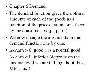
Properties of Demand Functions • Comparative statics analysis of ordinary demand functions -- the study of how Marshallian demands x1*(p1,p2,y) and x2*(p1,p2,y) change as prices p1, p2 and income y change.
Own-Price Changes • How does x1*(p1,p2,y) change as p1 changes, holding p2 and y constant? • Suppose only p1 increases, from p1’ to p1’’ and then to p1’’’.
Own-Price Changes Fixed p2 and y. x2 p1x1 + p2x2 = y p1 = p1’ x1
Own-Price Changes Fixed p2 and y. x2 p1x1 + p2x2 = y p1 = p1’ p1= p1’’ x1
Own-Price Changes Fixed p2 and y. x2 p1x1 + p2x2 = y p1 = p1’ p1=p1’’’ p1= p1’’ x1
Own-Price Changes Fixed p2 and y.
Own-Price Changes Fixed p2 and y. p1 = p1’ x1*(p1’)
p1 Own-Price Changes Fixed p2 and y. p1 = p1’ p1’ x1* x1*(p1’) x1*(p1’)
p1 Own-Price Changes Fixed p2 and y. p1 = p1’’ p1’ x1* x1*(p1’) x1*(p1’)
p1 Own-Price Changes Fixed p2 and y. p1 = p1’’ p1’ x1* x1*(p1’) x1*(p1’) x1*(p1’’)
p1 Own-Price Changes Fixed p2 and y. p1’’ p1’ x1* x1*(p1’) x1*(p1’’) x1*(p1’) x1*(p1’’)
p1 Own-Price Changes Fixed p2 and y. p1 = p1’’’ p1’’ p1’ x1* x1*(p1’) x1*(p1’’) x1*(p1’) x1*(p1’’)
p1 Own-Price Changes Fixed p2 and y. p1 = p1’’’ p1’’ p1’ x1* x1*(p1’) x1*(p1’’) x1*(p1’’’) x1*(p1’) x1*(p1’’)
p1 Own-Price Changes Fixed p2 and y. p1’’’ p1’’ p1’ x1* x1*(p1’) x1*(p1’’’) x1*(p1’’) x1*(p1’’’) x1*(p1’) x1*(p1’’)
p1 Own-Price Changes Demand curvefor commodity 1 Fixed p2 and y. p1’’’ p1’’ p1’ x1* x1*(p1’) x1*(p1’’’) x1*(p1’’) x1*(p1’’’) x1*(p1’) x1*(p1’’)
p1 Own-Price Changes Demand curvefor commodity 1 Fixed p2 and y. p1’’’ p1’’ p1’ x1* x1*(p1’) x1*(p1’’’) x1*(p1’’) x1*(p1’’’) x1*(p1’) x1*(p1’’)
p1 Own-Price Changes Demand curvefor commodity 1 Fixed p2 and y. p1’’’ p1’’ p1 price offer curve p1’ x1* x1*(p1’) x1*(p1’’’) x1*(p1’’) x1*(p1’’’) x1*(p1’) x1*(p1’’)
Own-Price Changes • The curve containing all the utility-maximizing bundles traced out as p1 changes, with p2 and y constant, is the p1- price offer curve. • The plot of the x1-coordinate of the p1- price offer curve against p1 is the demand curve for commodity 1.
Own-Price Changes • Usually we ask “Given the price for commodity 1 what is the quantity demanded of commodity 1?” • But we could also ask the inverse question “At what price for commodity 1 would a given quantity of commodity 1 be demanded?”
Own-Price Changes p1 Given p1’, what quantity isdemanded of commodity 1? p1’ x1*
Own-Price Changes p1 Given p1’, what quantity isdemanded of commodity 1?Answer: x1’ units. p1’ x1* x1’
Own-Price Changes p1 Given p1’, what quantity isdemanded of commodity 1?Answer: x1’ units. The inverse question is:Given x1’ units are demanded, what is the price of commodity 1? x1* x1’
Own-Price Changes p1 Given p1’, what quantity isdemanded of commodity 1?Answer: x1’ units. The inverse question is:Given x1’ units are demanded, what is the price of commodity 1? Answer: p1’ p1’ x1* x1’
Own-Price Changes • Taking quantity demanded as given and then asking what must be price describes the inverse demand function of a commodity.
Own-Price Changes A Cobb-Douglas example: is the demand function and is the inverse demand function.
Income Changes • How does the value of x1*(p1,p2,y) change as y changes, holding both p1 and p2 constant?
Income Changes Fixed p1 and p2. y’ < y’’ < y’’’
Income Changes Fixed p1 and p2. y’ < y’’ < y’’’
Income Changes Fixed p1 and p2. y’ < y’’ < y’’’ x2’’’ x2’’ x2’ x1’ x1’’’ x1’’
Income Changes Fixed p1 and p2. y’ < y’’ < y’’’ Incomeoffer curve x2’’’ x2’’ x2’ x1’ x1’’’ x1’’
Income Changes • A plot of quantity demanded against income is called an Engel curve.
Income Changes Fixed p1 and p2. y’ < y’’ < y’’’ Incomeoffer curve x2’’’ x2’’ x2’ x1’ x1’’’ x1’’
Income Changes Fixed p1 and p2. y’ < y’’ < y’’’ Incomeoffer curve y x2’’’ y’’’ x2’’ y’’ x2’ y’ x1’ x1’’’ x1’ x1’’’ x1* x1’’ x1’’
Income Changes Fixed p1 and p2. y’ < y’’ < y’’’ Incomeoffer curve y x2’’’ y’’’ Engelcurve; good 1 x2’’ y’’ x2’ y’ x1’ x1’’’ x1’ x1’’’ x1* x1’’ x1’’
Income Changes y Fixed p1 and p2. y’’’ y’’ y’ < y’’ < y’’’ y’ Incomeoffer curve x2’’’ x2’ x2* x2’’ x2’’’ x2’’ x2’ x1’ x1’’’ x1’’
Income Changes Engelcurve; good 2 y Fixed p1 and p2. y’’’ y’’ y’ < y’’ < y’’’ y’ Incomeoffer curve x2’’’ x2’ x2* x2’’ x2’’’ x2’’ x2’ x1’ x1’’’ x1’’
Income Changes Engelcurve; good 2 y Fixed p1 and p2. y’’’ y’’ y’ < y’’ < y’’’ y’ Incomeoffer curve x2’’’ x2’ x2* y x2’’ x2’’’ y’’’ Engelcurve; good 1 x2’’ y’’ x2’ y’ x1’ x1’’’ x1’ x1’’’ x1* x1’’ x1’’
Income Changes • In many examples the Engel curves have all been straight lines?Q: Is this true in general? • A: No. Engel curves are straight lines if the consumer’s preferences are homothetic.
Homotheticity • A consumer’s preferences are homothetic if and only iffor every k > 0. • That is, the consumer’s MRS is the same anywhere on a straight line drawn from the origin. p p Û (x1,x2) (y1,y2) (kx1,kx2) (ky1,ky2)
Income Effects • A good for which quantity demanded rises with income is called normal. • Therefore a normal good’s Engel curve is positively sloped.
Income Effects • A good for which quantity demanded falls as income increases is called income inferior. • Therefore an income inferior good’s Engel curve is negatively sloped.
Ordinary Goods • A good is called ordinary if the quantity demanded of it always increases as its own price decreases.
Ordinary Goods Fixed p2 and y. x2 x1
Ordinary Goods Fixed p2 and y. x2 p1 price offer curve x1
Ordinary Goods Fixed p2 and y. Downward-sloping demand curve x2 p1 p1 price offer curve Û Good 1 isordinary x1* x1
Giffen Goods • If, for some values of its own price, the quantity demanded of a good rises as its own-price increases then the good is called Giffen.
Ordinary Goods Fixed p2 and y. x2 p1 price offer curve x1
Ordinary Goods Demand curve has a positively sloped part Fixed p2 and y. x2 p1 p1 price offer curve Û Good 1 isGiffen x1* x1
Cross-Price Effects • If an increase in p2 • increases demand for commodity 1 then commodity 1 is a gross substitute for commodity 2. • reduces demand for commodity 1 then commodity 1 is a gross complement for commodity 2.