Introduction to Artificial Intelligence CS 438 Spring 2008

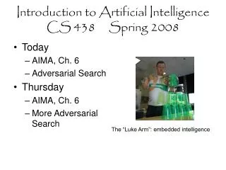
1. Introduction to Artificial IntelligenceCS 438 Spring 2008 • Today • AIMA, Ch. 6 • Adversarial Search • Thursday • AIMA, Ch. 6 • More Adversarial Search The “Luke Arm”: embedded intelligence

2. Why is game playing an interesting AI task? • Techniques used in game playing agents can be used in other problem solving tasks • Elements of uncertainty • Search space is too large to look at every possible consequence • Having an unpredictable opponent • Many games have a random element • Real-time decision making • Learning environment

3. Game Agents vs Human Champions • Chess – Deep Blue • defeated human world champion Garry Kasparov in a six-game match in 1997. Deep Blue searches 200 million positions per second, uses very sophisticated evaluation, and undisclosed methods for extending some lines of search up to 40 ply. • Checkers – Chinook • ended 40-year-reign of human world champion Marion Tinsley in 1994. Used a pre-computed endgame database defining perfect play for all positions involving 8 or fewer pieces on the board, a total of 444 billion positions. • Poker - Polaris • After two thousand hands and countless 'flops', 'rivers', and 'turns', two elite poker players, Phil "The Unabomber" Laak and Ali Eslami, have narrowly defeated Polaris. • Othello - Logistello • Scrabble - Quackle

4. Two Player Games Optimal Decisions • State Space Definition • Initial state • Board position and an indication of who goes first • Set of operators • All legal moves a play can make • Terminal (goal) test • Test to determine when the game is over • Utility function • Assigns a numeric value for the outcome of the game • Chess: +1 (win), 0 (draw), -1 (loss) • Backgammon: +192 to -192 • For multi-round games

5. Optimal Decisions • Min Max (minimax) Search • Always assume that your opponent is going to make the move that puts you in the worst possible situation, and conversely improves their own position as much as possible. • best achievable payoff against best play.

6. Minimax Search Tree

7. Minimax Steps • Generate search tree in depth first manner • Apply utility function to each terminal node • Use utility of terminal nodes to determine the utility of the node above • If the level above is your move (max) choose the maximum value of the leaf nodes • If the level above is your opponents move (min) choose minimum value of leaf nodes • Continue going back-up the tree assigning the utility value to each parent in a similar fashion • Once all of the states have been examined the utility of the best move will be assigned to the root.

8. Minimax • 4-ply game:

9. Minimax algorithm

10. Properties of minimax • Complete? Yes (if tree is finite) • Optimal? Yes (against an optimal opponent) • Time complexity? O(bm) • Space complexity? O(bm) (depth-first exploration) • For chess, b ≈ 35, m ≈100 for "reasonable" games exact solution completely infeasible

11. Resource limits • A move must be make in a time limit that does not allow the agent to search down to the terminal nodes • Suppose we have 100 secs, explore 104 nodes/sec106nodes per move • Standard approach: • cutoff test: • depth limit (perhaps add quiescence search) • evaluation function: Eval(s) • estimated desirability of position

12. Evaluation functions • Eval(s) • A numeric value indicating how good the chances of winning the game are from state s • Should be consistent with a utility function for the game • Largest value is a win, lowest value is a loss • Applied to the last level of state expanded • For chess, typically linear weighted sum of features Eval(s) = w1 f1(s) + w2 f2(s) + … + wn fn(s) • Weights are adjusted to improve play or new features could be added.

15. Hmmm, could you apply a similar idea to the peg board puzzle?