Download
1 / 33
330 likes | 371 Vues
Learn about receiver functions, methods to map time to depth, and advanced applications like velocity modeling and identifying layers of anisotropy and dip. Understand how to determine Vp/Vs and Moho depth, and correct move-out in seismic data interpretation.

E N D
Outline • Receiver Function Method • Mapping time to depth (Basic) • Advanced applicationsa. Determining Vp/Vs and Moho depthb. Velocity modelingc. Determining layers of anisotropy and dip
Receiver functions Receiver functions are used to isolate the response function that describes P-wave to S-wave conversions at horizontal velocity interfaces (layers) in the earth below the receiver (hence the name receiver function)
P-wave to S-wave conversions Frequency Domain h - horizontal v - vertical w - whitening
Forward Model (Convolution)Generation of recorded signal from Source and Earth Response source * response = signal = *
Inverse Model (Deconvolution )Using the signal and source to get the Earth Response function signal / source= response = / CASE OF NO NOISE! EVEN SMALL % OF NOISE CAN CREATE UNSTABLE SOLUTION – INVERSE THEORY and REGULARIZATIONTO SATBALIZE THE SOLUTION
Real Receiver function 3C Seismic Record: P-wave is the source (vertical)P-wave + converted S-wave are signal (isotropic-flat layer -> radial)
Outline • Receiver Function Method • Mapping time to depth (Basic) • Advanced applicationsa. Determining Vp/Vs and Moho depthb. Velocity modelingc. Determining layers of anisotropy and dip
Move-out correction and Mapping time to depth Want to know the timing difference between the direct P arrival (ts) and the converted S arrival (ts) as a function of depth. This can be done if we know the velocity of the wave-front in the vertical and horizontal directions P-wave x S-wave z tp ts
Move-out correction and Mapping time to depth Just a geometry problem! Tpds = ts – tp P-wave 1/Vpx S-wave 1/Vpz tp ts
Move-out correction and Mapping time to depth Just a geometry problem! The horizontal velocity is known, the rayparmeter - ‘p’ We need to know the P-velocity as a function of depth: Vp(z) And the ratio between Vp and Vs (Poisson’s ratio).
Move-out correction and Mapping time to depth How much do errors in assumptions affect the time to depth mapping? Vp(z) – An avg velocity difference of 6.2 and 6.5 translates to ~ 3 km at 70 km depth ie if the Moho is at 70 km and the crust has an avg velocity of 6.5 km/s, we use 6.2 km/s and compute a depth of ~ 67 km The horizontal velocity is known, the rayparmeter - ‘p’ We need to know the P-velocity as a function of depth: Vp(z) And the ratio between Vp and Vs (Poisson’s ratio).
Move-out correction and Mapping time to depth How much do errors in assumptions affect the time to depth mapping? Vp/Vs ratio – An avg difference of 1.72 to 1.79 translates to ~ 7 km at 70 km depth ie if the Moho is at 70 km and the crust has an avg Vp/Vs of 1.79, we use 1.72 to compute a depth of ~ 63 km The horizontal velocity is known, the rayparmeter - ‘p’ We need to know the P-velocity as a function of depth: Vp(z) And the ratio between Vp and Vs (Poisson’s ratio).
Data Coverage8/03 – 10/04 Teleseismic (blue) Distance 30-95 Deg Magnitude >=5.5 mb N - 179 Teleseismic Regional (Green) Distance <30 Deg Magnitude >=4.5 mb N - 571 Regional
Measurement of depth to Moho assuming Vp of 6.4 and Vp/Vs of 1.75
Outline • Receiver Function Method • Mapping time to depth (Basic) • Advanced applicationsa. Determining Vp/Vs and Moho depthb. Velocity modelingc. Determining layers of anisotropy and dip
Moho depth and Vp/Vs ratio If we assume Vp(z),we can write a function: H(Vp/Vs, D) = Tpms +Tppms + Tpsms which we can use to solve Vp/Vs and D Figures: Kennett, B
Example from station ES02 Moho depth 71 km Vp/Vs 1.77 Poisson’s 0.27 Pms + Ppms + Psms Pms + Ppms Depth below receiver (km) Vp/Vs ratio
Move-out correction and Mapping time to depth Just a geometry problem! Tppds = (ts – tp) + tp + tp = ts + tp P-wave 1/Vpx S-wave 1/Vpz tp ts
Move-out correction and Mapping time to depth Just a geometry problem! Tpsds = (ts – tp) + ts + tp = 2*ts P-wave 1/Vpx S-wave 1/Vpz
Examples from station ES34 Moho depth 65 km Vp/Vs 1.76 Poisson’s 0.26 Pms + Ppms + Psms Pms + Ppms Depth below receiver (km) Vp/Vs ratio