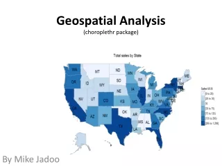
Geospatial Analysis (choroplethr package)
400 likes | 425 Vues
This seminar will provide an overview of geospatial analysis, including creating hypotheses, finding data sources, fixing data series, and using geographical statistics for analysis. Learn how to use the choroplethr package in R to generate geospatial maps.

Geospatial Analysis (choroplethr package)
E N D
Presentation Transcript
Geospatial Analysis(choroplethr package) By Mike Jadoo
Purpose • Bring about an awareness • Enable individuals to properly create analysis • Generate geospatial maps
R i386 3.2.3 (32 bit) * All packages associated with seminar is located at the top of the code file MAPS_R_CODE.txt
Geospatial Analysis • Geospatial analysis is applying statistical data to geographical locations in order to create inferences about a certain area using computer imagery.
Overview • Creating the hypothesis • Finding the data • Fixing/examining the data • Creating the map • Using geographical statistics for analysis
Hypothesis • Create the hypothesis - What are you trying to analyze or predict • Go over the topics relative theory -May involve extensive reading but it is the good first start!
Finding the data sources Government statistical agencies good starting point!! Can’t find the data your looking for? Call the agency. Staff is there to help. There are more providers of data, some have a cost.
Finding the data sources • Review the methodology, is this acceptable? • Make your own data • Scale • subdivision
Other method • Aggregate: may need to blend data sources • Disaggregate: using ratio’s of relevant data • Percentage change show growth over time
Fix data series • Missing observations - nearest neighbor - mean or median - interpolate
Geographical Statistics The study and practice of collecting, analyzing, and presenting data that has a geographic or areal dimension.
Statistics Old statistical measures with a new exploratory ability • Skewness: measures the degree of symmetry in a distribution • Kutursis: measures the degree of shape (flatness or peakedness) of the data series [OLD]
Statistics Old statistical measures with a new exploratory ability • Skewness: if an area shows a level of skewness this means that there are subdivisions that is experiences outliers • Kurtosis: can signal if there are clusters (peaks) of points in an area [NEW]
Skewness Kurtosis Statistical inferences Geographical inferences
Geographical Statistics • Coefficient Variation: amount of variation in spatial patterns relative measure of dispersion • Individual deviation
Geographical Statistics • Mean Deviation
Data Structure • Example of imported table: County tableState table
Creating the map • Which map do you want to make and how many? -Depends on what are you are analyzing -Match series with Long/Lat, state and county FIPS code, or zip codes
Creating the map • Some examples using R- Map subdivision • US map with state lines • US map with county lines • State map with county lines • Maps with zip codes lines
US national map state lines Starter code: library(choroplethr) newdata<-read.csv("E:/COURSE_MATERIAL2/GEO_SPACE/BEA.csv") state_choropleth(newdata, title = "GDP by STATE“, legend = "US $")
US national map county lines Starter code: newdata<-read.csv("E:/COURSE_MATERIAL2/GEO_SPACE/CTY_MAY_MAP_R.csv") county_choropleth(newdata,title="Total Sales in May", legend="Sales $", num_colors=1)
State Map and county lines Starter code: library(choroplethr) newda2ta<-read.csv("E:/COURSE_MATERIAL2/GEO_SPACE/CTY_TOT_SALES_MAP_R.csv") county_choropleth(newda2ta, state_zoom="illinois", title = "Statistical Seminars Rock", legend = "Sales",)
County map with Google ref Starter code: library(choroplethrMaps) data(county.regions) data(df_pop_county) county_choropleth(df_pop_county, title = "Population of Counties in New York City", legend = "Population", num_colors = 1, county_zoom = 36047, reference_map = TRUE)
US state map zip code lines Starter code: library(devtools) install_github('arilamstein/choroplethrZip@v1.4.0') library(choroplethrZip) data(df_pop_zip) df_pop_zip zip_choropleth(df_pop_zip, state_zoom="new york", title=" New York State map US Census Population Estimates", legend="Population")
US county map with zip code lines and Google ref Starter code: library(devtools) install_github('arilamstein/choroplethrZip@v1.4.0') library(choroplethrZip) data(df_pop_fips) nyc_fips = c(36005, 36047, 36061, 36081, 36085) zip_choropleth(df_pop_zip, county_zoom=nyc_fips, title="New York City map US Census Population Estimates", legend="Population", reference_map=TRUE)
Key Highlights • Outliers • Strange situations in certain areas
Outliers Starter code (Ari): library(ggplot2) highlight_county = function(county_fips) { library(choroplethrMaps) data(county.map, package="choroplethrMaps", envir=environment()) df = county.map[county.map$region %in% county_fips, ] geom_polygon(data=df, aes(long, lat, group = group), color = "red", fill = NA, size = 1) } library(ggplot2) choro_outlier = county_choropleth(newda2ta, state_zoom="california", title="Highest Sales", num_colors=1) + highlight_county(6037)
Adjacent Counties Analysis Go to US Census site official list adjacent counties Starter code: n_fips = c(1011, 1045, 1067, 1109, 1113,13061,13239,13259) county_choropleth(newdata, county_zoom= n_fips, title="Total Sales in May", legend="Sales $", num_colors=1, reference_map = TRUE)
Spatial Autocorrelation Measures the degree of areas associated data values tendency to be clustered together First Law of Geography (Tobler’s Law): everything depends on everything else, but closer things more so
Spatial autocorrelation • Global measures of analysis • Local measures of analysis
Spatial autocorrelation ** TECHNICAL NOTE** • If using the spdep package coordinates needs to be converted first to neighbors list [nb] then to spatial weight [listw]- (Anselin)
Global Spatial Autocorrelation Identify and measure the whole area examined and doesn’t describe individual subsections (Murack) • Cluster analysis (Moran I) • Hot spot analysis (GETIS-ORD Gi*)
Global Spatial Autocorrelation moran.test(newdata3$Av8top,nb2listw(boi)) #OUTPUT: Moran I test under randomisation data: newdata3$Av8top weights: nb2listw(boi) Moran I statistic standard deviate = 2.24, p-value = 0.01255 alternative hypothesis: greater sample estimates: Moran I statistic Expectation Variance 0.2314795 -0.1111111 0.0233917 • Cluster analysis (Moran I) • Hot spot analysis (GETIS-ORD Gi*) globalG.test(newdata3$Av8top,nb2listw(boi, style="B")) #OUTPUT: Getis-Ord global G statistic data: newdata3$Av8top weights: nb2listw(boi, style = "B") standard deviate = -0.94197, p-value = 0.8269 alternative hypothesis: greater sample estimates: Global G statistic Expectation Variance 0.502741777 0.533333333 0.001054695
Local Indicators of Spatial Autocorrelation Analyzes the specific areas within a group • Cluster analysis (Moran I) • Hot spot analysis (GETIS-ORD Gi*)
Local Indicators of Spatial Autocorrelation • Moran I localmoran(newdata3$Av8top,nb2listw(boi)) #OUTPUT: Ii E.Ii Var.Ii Z.Ii Pr(z > 0) 1 -0.09693758 -0.1111111 0.14710649 0.03695407 0.485260815 2 -0.00270023 -0.1111111 0.06653806 0.42027912 0.337140783 3 0.76302485 -0.1111111 0.14710649 2.27909835 0.011330610 4 0.21848568 -0.1111111 0.22767493 0.69075713 0.244859089 5 0.09329253 -0.1111111 0.22767493 0.42838181 0.334186583 6 0.64928782 -0.1111111 0.09876543 2.41957458 0.007769337 7 0.11005317 -0.1111111 0.04351851 1.06017607 0.144532253 8 0.08226948 -0.1111111 0.04351851 0.92699178 0.176965402 9 -0.22974551 -0.1111111 0.04351851 -0.56868747 0.715215874 10 0.72776515 -0.1111111 0.38881179 1.34532804 0.089259662 attr(,"call") localmoran(x = newdata3$Av8top, listw = nb2listw(boi)) attr(,"class") [1] "localmoran" "matrix"
Local Indicators of Spatial Autocorrelation • GETIS-ORD Gi* localG(newdata3$Av8top,nb2listw(boi)) #OUTPUT: [1] 0.06782567 -0.05793132 -1.98996426 0.65987906 0.82076260 -2.13377740 [7] -1.61158181 -1.00055525 -1.78151210 1.12463577 attr(,"gstari") [1] FALSE attr(,"call") localG(x = newdata3$Av8top, listw = nb2listw(boi)) attr(,"class") [1] "localG"
L.I.S.A • These statistics can make analysis more valuable when using maps and spatial data • More information can be derived which can bring about more discoveries
Recap • Approaching analysis building-hypothesis • Finding/fixing data • New interpretations of statistical measures • Creating Maps • Using geographical statistics to create new analysis
Special Thanks • Ari Lamstein- choroplethr package