
Information Extraction using HMMs
E N D
Presentation Transcript
Information Extraction using HMMs Sunita Sarawagi
Title Journal Year Author Volume Page IE by text segmentation Source: concatenation of structured elements with limited reordering and some missing fields • Example: Addresses, bib records House number Zip State Building Road City 4089 Whispering Pines Nobel Drive San Diego CA 92122 P.P.Wangikar, T.P. Graycar, D.A. Estell, D.S. Clark, J.S. Dordick (1993) Protein and Solvent Engineering of Subtilising BPN' in Nearly Anhydrous Organic Media J.Amer. Chem. Soc. 115, 12231-12237.
0.5 0.9 0.5 0.1 0.8 0.2 Hidden Markov Models A C 0.6 0.4 • Doubly stochastic models • Efficient dynamic programming algorithms exist for • Finding Pr(S) • The highest probability path P that maximizes Pr(S,P) (Viterbi) • Training the model • (Baum-Welch algorithm) A C 0.9 0.1 S1 S2 S4 S3 A C 0.3 0.7 A C 0.5 0.5
Input features • Content of the element • Specific keywords like street, zip, vol, pp, • Properties of words like capitalization, parts of speech, number? • Inter-element sequencing • Intra-element sequencing • Element length • External database • Dictionary words • Semantic relationship between words • Frequency constraints
Y A C X B Z A B C 0.1 0.1 0.8 0.4 0.2 0.4 0.6 0.3 0.1 Emission probabilities Transition probabilities 0.5 0.9 0.5 0.1 0.8 0.2 dddd dd 0.8 0.2 IE with Hidden Markov Models • Probabilistic models for IE Title Author Journal Year
HMM Structure • Naïve Model: One state per element • Nested model Each element another HMM
Comparing nested models • Naïve: Single state per tag • Element length distribution: a, a2, a3,… • Intra-tag sequencing not captured • Chain: • Element length distribution: • Each length gets its own parameter • Intra-tag sequencing captured • Arbitrary mixing of dictionary, • Eg. “California York” • Pr(W|L) not modeled well. • Parallel path: • Element length distribution: each length gets a parameter • Separates vocabulary of different length elements, (limited bigram model)
Bigram model of Bikel et al. • Each inner model a detailed bigram model • First word: conditioned on state and previous state • Subsequent words conditioned on previous word and state • Special “start” and “end” symbols that can be thought • Large number of parameters • (Training data order~60,000 words in the smallest experiment) • Backing off mechanism to previous simpler “parent” models (lambda parameters to control mixing)
Building name S1 S2 Prefix Suffix S4 S3 Separate HMM per tag • Special prefix and suffix states to capture the start and end of a tag Road name S1 S2 Prefix Suffix S4
HMM Dictionary • For each word (=feature), associate the probability of emitting that word • Multinomial model • Features of a word, • example, • part of speech, • capitalized or not • type: number, letter, word etc • Maximum entropy models (McCallum 2000), other exponential models • Bikel: <word,feature> pairs
Learning model parameters • When training data defines unique path through HMM • Transition probabilities • Probability of transitioning from state i to state j = number of transitions from i to j total transitions from state i • Emission probabilities • Probability of emitting symbol k from state i = number of times k generated from i number of transition from I • When training data defines multiple path: • A more general EM like algorithm (Baum-Welch)
Smoothing • Two kinds of missing symbols: • Case-1: Unknown over the entire dictionary • Case-2: Zero count in some state • Approaches: • Laplace smoothing: ki + 1 m + |T| • Absolute discounting • P(unknown) proportional to number of distinct tokens • P(unknown) = (k’) x (number of distinct symbols) • P(known) = (actual probability)-(k’), • k’ is a small fixed constant, case 2 smaller than case 1
Smoothing (Cont.) • Smoothing parameters derived from data • Partition training data into two parts • Train on part-1 • Use part-2 to map all new tokens to UNK and treat it as new word in vocabulary • OK for case-1, not good for case-2. Bikel et al use this method for case-1. For case-2 zero counts are backed off to 1/(Vocab-size)
Using the HMM to segment • Find highest probability path through the HMM. • Viterbi: quadratic dynamic programming algorithm 115 Grant street Mumbai 400070 115 Grant ……….. 400070 House House House House Road Road Road Road City City City ot ot Pin Pin Pin Pin
Most Likely Path for a Given Sequence • The probability that the path is taken and the sequence is generated: transition probabilities emission probabilities
begin end Example 0.4 0.2 A 0.4 C 0.1 G 0.2 T 0.3 A 0.2 C 0.3 G 0.3 T 0.2 0.8 0.6 0.5 1 3 0 5 A 0.4 C 0.1 G 0.1 T 0.4 A 0.1 C 0.4 G 0.4 T 0.1 0.5 0.9 0.2 2 4 0.1 0.8
Finding the most probable path: the Viterbi algorithm • define to be the probability of the most probable path accounting for the first i characters of x and ending in state k • we want to compute , the probability of the most probable path accounting for all of the sequence and ending in the end state • can define recursively • can use dynamic programming to find efficiently
Finding the most probable path: the Viterbi algorithm • initialization:
The Viterbi algorithm • recursion for emitting states (i =1…L): keep track of most probable path
The Viterbi algorithm • to recover the most probable path, follow pointers back starting at • termination:
Database Integration • Augment dictionary • Example: list of Cities • Assigning probabilities is a problem • Exploit functional dependencies • Example • Santa Barbara -> USA • Piskinov -> Georgia
House number City State Area Road Name 2001 University Avenue, Kendall Sq., Piskinov, Georgia House number Area City Country Road Name 2001 University Avenue, Kendall Sq., Piskinov, Georgia 2001 University Avenue, Kendall Sq. Piskinov, Georgia
Frequency constraints • Including constraints of the form: the same tag cannot appear in two disconnected segments • Eg: Title in a citation cannot appear twice • Street name cannot appear twice • Not relevant for named-entity tagging kinds of problems
Constrained Viterbi Original Viterbi Modified Viterbi ….
Comparative Evaluation • Naïve model – One state per element in the HMM • Independent HMM – One HMM per element; • Rule Learning Method – Rapier • Nested Model – Each state in the Naïve model replaced by a HMM
Results: Comparative Evaluation The Nested model does best in all three cases (from Borkar 2001)
Results: Effect of Feature Hierarchy Feature Selection showed at least a 3% increase in accuracy
Results: Effect of training data size HMMs are fast Learners. We reach very close to the maximum accuracy with just 50 to 100 addresses
HMM approach: summary Inter-element sequencing Intra-element sequencing Element length Characteristic words Non-overlapping tags • Outer HMM transitions • Inner HMM • Multi-state Inner HMM • Dictionary • Global optimization