From hydrological concepts to a numerical model
220 likes | 377 Vues
Short course on “ Model building, inference and hypothesis testing in hydrology ” 21-25 May, 2012. From hydrological concepts to a numerical model. Martyn Clark. Approach. Stick to very simple (yet robust) numerical methods Simpler than those presented in “Numerical Recipes”

From hydrological concepts to a numerical model
E N D
Presentation Transcript
Short course on “Model building, inference and hypothesis testing in hydrology” 21-25 May, 2012 From hydrological concepts to a numerical model Martyn Clark
Approach • Stick to very simple (yet robust) numerical methods • Simpler than those presented in “Numerical Recipes” • Yet very easy for people to code from scratch, and retrofit existing hydrologic models • Learn by doing • “I never really understand something until I code it up myself” • Exercises to implement the methods that are introduced • Encourage discussion
Perceptual Model Understanding of the Earth System Not constrained by mathematics Different for different people (based on training, experience) Conceptual Model Synthesis (simplification) of the perceptual model Requires specifying System boundaries Relevant inputs, state variables and outputs Physical laws to be obeyed and simplifying assumptions Different conceptual models = different hypotheses of system behavior Numerical Model Temporal integration of the governing model equations The typical hydrologic modeling recipe
Outline • Numerical methods for bucket-style hydrologic models • The explicit Euler method • The implicit Euler method • Adaptive sub-stepping • Ad-hoc numerical implementations in hydrologic models • Exploring impacts of unreliable numerical implementation • Macro-scale and micro-scale discontinuities in model response surfaces and associated difficulties in model calibration and sensitivity analyses • Computational cost • Fragility of unreliable numerical implementations in predictive mode • Summary and outlook
The exact solution of the ODE system (and the need for approximations) • The ODE system from Clark et al. (2008) can be written as • The exact solutionof the average flux over the interval tn (start of the time step) to tn+1 (end of the time step) is • Given an estimateof the average flux, the model state variables can be temporally integrated as • The exact solution is computationally expensive, so approximations to the exact solution are used • The approximation controls the stability, accuracy, smoothness, and efficiency of the solution
The bread and butter of hydrology:The explicit Euler method • The most straightforward approximation to the exact solution is the explicit Euler method where the flux at the start of the time step is used to approximate the average flux over the time step • The explicit Euler method linearly extrapolates from the initial condition along the initial slope of g(S)
Try this… • A famous hydrologist (weight = 90 kg) has decided to go skydiving, and has asked you to determine how fast they will fall. • The hydrologist in question thinks that it is acceptable for you to use Newton’s second law of motion considering only the gravitational force (Fgrav) and the force due to air resistance (Fres) . That is, where m = mass (kg) and v is the fall velocity (m s-1). • Further, the hydrologist pursues the paradigm of parsimony, and is quite happy for you to use an empirical representation of the resistance force. After some discussion, you agree that the terms on the right-hand-side can be written as where k is a proportionality constant (for freefall, assume k = 15 kg s-1), and g is the gravitational acceleration 9.81 m s-2). • Your mission, should you choose to accept it:Based on an initial velocity of zero (the hydrologist is hopping out of a hovering helicopter), temporally integrate the ODE for a 3 minute period using the explicit Euler method with 10 second time steps.
The parachute problem (freefall) • ODE: • Constants: • m = mass of the hydrologist (90 kg) • g = gravitational acceleration (9.81 m s-2) • k = proportionality constant for freefall (15 kg s-1) • Hence • Numerical approximation: explicit Euler • Length of time step: Δt = 10 seconds • Initial velocity = zero m s-1 • the hydrologist is hopping out of a hovering helicopter
Let’s see if we can do better… SOLVE THE PROBLEM AGAIN, EXCEPT THIS TIME USE THE EXPLICIT EULER METHOD WITH A TIME STEP OF 0.1 SECONDS
The parachute problem (landing) • Velocity ODE: • Position ODE: • Initial conditions: • v = initial velocity (terminal velocity from the freefall example = 58 m s-1) • z = height to open the parachute (500 m) • Use the same constants as in the freefall example, except for k: • m = mass of the hydrologist (90 kg) • g = gravitational acceleration (9.81 m s-2) • k = proportionality constant for the open chute(250 kg s-1) • Numerical approximation: explicit Euler with Δt = 10 seconds
Poor numerical implementation can be downright dangerous! Far out dude… I think that guy just tomatoed!
Once again, short steps save the day… Terminal velocity = 3.53 m/s = 12.71 km/hr = 7.89 mi/hr
Can we do better than the explicit Euler method?Can we both increase accuracy and decrease computing costs?
The implicit Euler method • Approximates the exact solution of the average flux by estimating the flux at the end of the time step • The implicit Euler method requires that the computed flux at the end of the time step is consistent with the estimated solution: • In general, this requires iteration and can be computationally expensive.
Newton-Raphson iteration • The Newton-Raphson method finds the root of a function by evaluating the function f (x) and the function derivatives f ́ (x) at arbitrary points of x. • The function:In the implicit Euler method f (x) is the residual between a trial state variable (x) and the solution at the end of the time step estimated using the trial value x: • The derivative:The derivative f ́ (x) can be computed using finite differences, as • The new value of x can then be computed as and iterate until either the function or the derivative are below a user-specified error tolerance
Let’s give it a go:Can the implicit Euler method save our famous hydrologist? • Step 1: • Provide an initial guess of v (vm) • Compute the function evaluation (the residual) at vm and vm+ɛ • requires the derivatives g(vm) and g(vm+ɛ) • Notation: m=iteration index, and n=time step index; n denotes the start of the time step, and v0 is the initial guess of v • Compute the derivative of the function evaluation • Step 2: compute a new estimate of v and go back to step one, replacing the initial guess of v with thenew estimate of v • Keep going until you are happy!
Summary and outlook • In many cases model analysis complexities are consequences of numerical artifacts in the model implementation • Numerical errors of uncontrolled time stepping schemes routinely dwarf the structural errors of the model conceptualization • The robust numerics paradigm is yet to be accepted as the required standard in conceptual hydrology • Reliable hydrologic modeling is a major challenge without adding confounding numerical artifacts—let’s avoid preventable numerical troubles before tackling more genuine challenges!