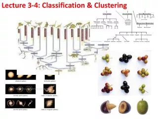
Lecture 3-4: Classification & Clustering

1. Lecture 3-4: Classification & Clustering

2. Both operate a partitioning of the parameterspace. Clustering: predictivevalueClassification: descriptivevalue

3. Both clustering and classification aim at partitioning a dataset into subsets that bear similar characteristics. Different to classification clustering does not assume any prior knowledge, which are the classes/clusters to be searched for. Class label attributes (even when they do exist) are not used in the training phase. Clustering serves in particular for exploratory data analysis with little or no prior knowledge. Classification requires samples of templates (i.e. sets of objects with well measured target value). This set is also called Knowledge Base (KB)

4. Inter-cluster distances are maximized Intra-cluster distances are minimized • Logical structure of a Clustering problem • Given: database D with N d-dimensional data items • Find: partitioning into k clusters and noise • • A good clustering method will produce high quality clusters with • – high intra-classsimilarity • – low inter-classsimilarity • The quality of a clustering result depends on both the similarity measure used by the method and its implementation

5. How many clusters? Six Clusters Two Clusters Four Clusters Notion of Cluster can be Ambiguous

6. A Partitional Clustering Types of Clusterings • Important distinction between hierarchical and partitionalsets of clusters • Partitional Clustering • A division data objects into non-overlapping subsets (clusters) such that each data object is in exactly one subset • Hierarchical clustering • A set of nested clusters organized as a hierarchical tree Original Points

7. Hierarchical Clustering Traditional Hierarchical Clustering Traditional Dendrogram Non-traditional Hierarchical Clustering Non-traditional Dendrogram

8. Other Distinctions Between Sets of Clusters • Exclusive versus non-exclusive • In non-exclusive clusterings, points may belong to multiple clusters. • Can represent multiple classes or ‘border’ points • Fuzzy versus non-fuzzy • In fuzzy clustering, a point belongs to every cluster with some weight between 0 and 1 • Weights must sum to 1 • Probabilistic clustering has similar characteristics • Partial versus complete • In some cases, we only want to cluster some of the data • Heterogeneous versus homogeneous • Cluster of widely different sizes, shapes, and densities

9. Types of Clusters • Well-separated clusters • Center-based clusters • Contiguous clusters • Density-based clusters • Property or Conceptual • Described by an Objective Function

10. Types of Clusters: Well-Separated • Well-Separated Clusters: • A cluster is a set of points such that any point in a cluster is closer (or more similar) to every other point in the cluster than to any point not in the cluster. 3 well-separated clusters

11. Types of Clusters: Center-Based • Center-based • A cluster is a set of objects such that an object in a cluster is closer (more similar) to the “center” of a cluster, than to the center of any other cluster • The center of a cluster is often a centroid, the average of all the points in the cluster, or a medoid, the most “representative” point of a cluster 4 center-based clusters

12. Types of Clusters: Contiguity-Based • Contiguous Cluster (Nearest neighbor or Transitive) • A cluster is a set of points such that a point in a cluster is closer (or more similar) to one or more other points in the cluster than to any point not in the cluster. 8 contiguous clusters

13. Types of Clusters: Density-Based • Density-based • A cluster is a dense region of points, which is separated by low-density regions, from other regions of high density. • Used when the clusters are irregular or intertwined, and when noise and outliers are present. 6 density-based clusters

14. Types of Clusters: Conceptual Clusters • Shared Property or Conceptual Clusters • Finds clusters that share some common property or represent a particular concept. . 2 Overlapping Circles

15. Clustering isessentially a projection business: (find the projection(featurereduction) whichminimizes the distance/similaritybetween data points)

16. Questions to askbeforepicking up a method • Quantitative Criteria • Scalability: number of data objects N • High dimensionality • We want to deal with large and complex (high D) data sets. High D increases sparseness of the data. The number of choices for projection dimensionsgrowscombinatorially with D. • Qualitative criteria • Ability to deal with different types of attributes • Discovery of clusters with arbitrary shape • Addresses the ability of dealing with continuous as well as • categorical attributes, and the type of clusters that can be found. • Many clustering methods can detect only very simple geometrical shapes, like spheres, hyperplanes, hyperspheres, ellipsoids, etc.

17. Robustness • Able to deal with noise and outliers • Insensitive to order of input records • Clustering methods can be sensitive both to noisy data and the order of how the records are processed. In both cases it would be undesireable to have a dependency of the clustering result on these aspects which are unrelated to the nature of data in question. • Usage-orientedcriteria • Incorporationof user-specifiedconstraints • Interpretability and usability • a clustering method can incorporate user requirements both in terms of information that is provided from the user to the clustering method (in terms of constraints), which can guide the clustering process, and in terms of what information is provided from the method to the user.

18. PartitioningMethodsare a basic approach to clustering. • Partitioning methods attempt to partition the data set into a given number k of clusters optimizing intracluster similarity and inter-cluster dissimilarity. • Construct a partition of a database D of n objects into a set of k clusters, k predefined. • Given k, find a partition of k clusters that optimizes the chosen • Partitioningcriterion • Globally optimal: exhaustively enumerate all partitions • Heuristic methods: k-means and k-medoids algorithms • k-means: each cluster is represented by the center of the cluster • k-medoidsor PAM (Partition around medoids): each cluster is represented by one of the objects in the cluster

19. Types of Clusters: Objective Function • Clusters Defined by an Objective Function • Finds clusters that minimize or maximize an objective function. • Enumerate all possible ways of dividing the points into clusters and evaluate the `goodness' of each potential set of clusters by using the given objective function. (NP Hard) • Can have global or local objectives. • Hierarchical clustering algorithms typically have local objectives • Partitional algorithms typically have global objectives • A variation of the global objective function approach is to fit the data to a parametrized data model. • Parameters for the model are determined from the data. • Mixture models assume that the data is a ‘mixture' of a number of statistical distributions.

20. Types of Clusters: Objective Function … • Map the clustering problem to a different domain and solve a related problem in that domain • Proximity matrix defines a weighted graph, where the nodes are the points being clustered, and the weighted edges represent the proximities between points • Clustering is equivalent to breaking the graph into connected components, one for each cluster. • Want to minimize the edge weight between clusters and maximize the edge weight within clusters

21. Characteristics of the Input Data Are Important • Type of proximity or density measure • This is a derived measure, but central to clustering • Sparseness • Dictates type of similarity • Adds to efficiency • Attribute type • Dictates type of similarity • Type of Data • Dictates type of similarity • Other characteristics, e.g., autocorrelation • Dimensionality • Noise and Outliers • Type of Distribution

22. The k-MeansPartitioningMethod Assume objects are characterized by a d-dimensional vector Given k, the k-means algorithm is implemented in 4 steps Step 1: Partition objects into k nonempty subsets Step 2: Compute seed points as the centroids of the clusters of the current partition. The centroid is the center (mean point) of the cluster. Step 3: Assign each object to the cluster with the nearest seed point Step 4: Stop when no new assignment occurs, otherwise go back to Step 2

24. Properties of k-Means • Strengths • Relatively efficient: O(tkn), where n is # objects, k is # clusters, and t is # iterations. Normally, k, t << n. • Often terminates at a local optimum, depending on seed point • The global optimum may be found using techniques such as: deterministic annealingand geneticalgorithms • Weaknesses • Applicable only when mean is defined, therefore not applicable to categorical data • Need to specify k, the number of clusters, in advance • Unable to handle noisy data and outliers • Not suitable to discover clusters with non-convex shapes

25. Optimal Clustering Sub-optimal Clustering Two different K-means Clusterings Original Points

26. Importance of Choosing Initial Centroids

27. Importance of Choosing Initial Centroids

28. Evaluating K-means Clusters • Most common measure is Sum of Squared Error (SSE) • For each point, the error is the distance to the nearest cluster • To get SSE, we square these errors and sum them. • x is a data point in cluster Ciand mi is the representative point/center for cluster Ci • Given two clusters, we can choose the one with the smallest error • One easy way to reduce SSE is to increase K, the number of clusters • A good clustering with smaller K can have a lower SSE than a poor clustering with higher K

29. Problems with Selecting Initial Points • If there are K ‘real’ clusters then the chance of selecting one centroid from each cluster is small (decreases with K) • If clusters are the same size, n, then • For example, if K = 10, then probability = 10!/1010 = 0.00036 • Sometimes the initial centroids will readjust themselves in ‘right’ way, and sometimes they don’t • Consider an example of five pairs of clusters

30. 10 Clusters Example Starting with two initial centroids in one cluster of each pair of clusters

31. 10 Clusters Example Starting with two initial centroids in one cluster of each pair of clusters

32. 10 Clusters Example Starting with some pairs of clusters having three initial centroids, while other have only one.

33. Solutions to Initial Centroids Problem • Multiple runs • Helps, but probability is not on your side • Sample and use hierarchical clustering to determine initial centroids • Select more than k initial centroids and then select among these initial centroids • Select most widely separated • Postprocessing • Bisecting K-means • Not as susceptible to initialization issues

34. Handling Empty Clusters • Basic K-means algorithm can yield empty clusters • Several strategies • Choose the point that contributes most to SSE • Choose a point from the cluster with the highest SSE • If there are several empty clusters, the above can be repeated several times.

35. Updating Centers Incrementally • In the basic K-means algorithm, centroids are updated after all points are assigned to a centroid • An alternative is to update the centroids after each assignment (incremental approach) • Each assignment updates zero or two centroids • More expensive • Introduces an order dependency • Never get an empty cluster • Can use “weights” to change the impact

36. Pre-processing and Post-processing • Pre-processing • Normalize the data • Eliminate outliers • Post-processing • Eliminate small clusters that may represent outliers • Split ‘loose’ clusters, i.e., clusters with relatively high SSE • Merge clusters that are ‘close’ and that have relatively low SSE • Can use these steps during the clustering process • ISODATA

37. Limitations of K-means • K-means has problems when clusters are of differing • Sizes • Densities • Non-globular shapes • K-means has problems when the data contains outliers.

38. Limitations of K-means: Differing Sizes K-means (3 Clusters) Original Points

39. Limitations of K-means: Differing Density K-means (3 Clusters) Original Points

40. Limitations of K-means: Non-globular Shapes Original Points K-means (2 Clusters)

41. Overcoming K-means Limitations Original Points K-means Clusters • One solution is to use many clusters. • Find parts of clusters, but need to put together.

42. Overcoming K-means Limitations Original Points K-means Clusters

43. Overcoming K-means Limitations Original Points K-means Clusters

44. Hierarchical Clustering • Produces a set of nested clusters organized as a hierarchical tree • Can be visualized as a dendrogram • A tree like diagram that records the sequences of merges or splits

45. Strengths of Hierarchical Clustering • Do not have to assume any particular number of clusters • Any desired number of clusters can be obtained by ‘cutting’ the dendogram at the proper level • They may correspond to meaningful taxonomies • Example in biological sciences (e.g., animal kingdom, phylogeny reconstruction, …)

46. Hierarchical Clustering • Two main types of hierarchical clustering • Agglomerative: • Start with the points as individual clusters • At each step, merge the closest pair of clusters until only one cluster (or k clusters) left • Divisive: • Start with one, all-inclusive cluster • At each step, split a cluster until each cluster contains a point (or there are k clusters) • Traditional hierarchical algorithms use a similarity or distance matrix • Merge or split one cluster at a time

47. Agglomerative Clustering Algorithm • More popular hierarchical clustering technique • Basic algorithm is straightforward • Compute the proximity matrix • Let each data point be a cluster • Repeat • Merge the two closest clusters • Update the proximity matrix • Until only a single cluster remains • Key operation is the computation of the proximity of two clusters • Different approaches to defining the distance between clusters distinguish the different algorithms

48. p1 p2 p3 p4 p5 . . . p1 p2 p3 p4 p5 . . . How to Define Inter-Cluster Similarity Similarity? • MIN • MAX • Group Average • Distance Between Centroids • Other methods driven by an objective function • Ward’s Method uses squared error Proximity Matrix

49. p1 p2 p3 p4 p5 . . . p1 p2 p3 p4 p5 . . . How to Define Inter-Cluster Similarity • MIN • MAX • Group Average • Distance Between Centroids • Other methods driven by an objective function • Ward’s Method uses squared error Proximity Matrix

50. p1 p2 p3 p4 p5 . . . p1 p2 p3 p4 p5 . . . How to Define Inter-Cluster Similarity • MIN • MAX • Group Average • Distance Between Centroids • Other methods driven by an objective function • Ward’s Method uses squared error Proximity Matrix