Ozone transport network
210 likes | 327 Vues
Analyzing the transport of East Asian Dust across the Pacific in the 1998 event, focusing on California's complex ozone transport network. Understanding local and transported ozone contributions, methodologies for analysis, and connecting the network to air pollution management. Leveraging data from California's air monitoring network and referencing ozone transport studies to optimize pollution control strategies.

Ozone transport network
E N D
Presentation Transcript
Ozone transportnetwork GuoxunTian CS 790G Fall 2010
Overview • Introduction • My goal and Problems • Methodology • Two way to solve the problems • How to connect this network to our course? • Where my data come from? • Reference • Questions
Transport of East Asian Dust across the pacific April 1998 event R. Husar et al.(1998) http://en.wikipedia.org/wiki/File:Chinadustmovie.gif http://en.wikipedia.org/wiki/File:Dust_movie.gif
Why California • California has the highest ozone level
My goal • Goal: to build a complex network of ozone transport based on 15 basins California is divided into 15 Air Basins to better manage air pollution. Air basin boundaries were decided by grouping similar geographic features together. Some air basins really are like a basin, with valleys surrounded by mountains. Political boundaries, Such as counties, were also important. • In this network, the nodes represent all basins and the edges represent the ozone transportation between them.
My goal Air pollution emissions from one air basin are often blown into a neighbor’s air basin
Problems Local Ozone Local ozone concentrations = Natural ozone + Transported ozone(generated from emissions from upwind cities and natural events such as wildfires) + Local ozone(generated from local anthropogenic emissions)
Problems (1 of 2) • Background ozone • What is the typical natural background ozone concentration? • Transport • How much ozone, above natural background, was transported into each city or basin? • What are the typical source areas for transported ozone?
Problems (2 of 2) • Local contribution • What amount of locally generated ozone was produced at each city? • Contribution comparison • On what percentage of high-ozone days was peak local 8-hr ozone dominated by locally generated ozone compared to transported ozone? • How do these percentages change for each city by transport direction? • How do the contribution amounts compare among the cities?
Methodology 1. Statistcal Analyses Analyses of the time of peak ozone concentration at various monitoring sites can yield useful information on transport patterns and source areas. B Morning A In most major source areas of interest in California, transport winds are light in the morning, allowing ozone precursor concentrations to build up and zone to form. B A Wind
Methodology 2. Back trajectory analysis Back trajectory analyses are computer models based on data from past weather forecasting models that predict how air moves and arrives at a fixed destination (Yarwood et al., 2000). The National Oceanic and Atmospheric Administration (NOAA) provides a modeling tool known as the HYSPLIT model, which calculates back trajectories. Another tool that calculates back trajectories, VIEWS, provides a similar product using different assumptions and weather models. These tools can be used as indicators as to whether or not a high ozone level could be attributed to ozone transport from other areas (Yarwood et al., 2000).
Methodology Peak Local Ozone = Incoming (natural background + transported anthropogenic) + Local Anthropogenic • System developed to calculate incoming ozone (Clinton P. MacDonald) • Ran multiple backward trajectories each day for five years (2001–2005, April–October); • Determined the daily peak 8-hr ozone concentration at the last site near which each trajectory passed during daylight hours prior to entering each city; and • Averaged all concentrations to estimate incoming boundary layer concentration each day.
How to connect this network to our course? Ozone Transport sketch map of San Francisco Bay Area Air Basin Do analysis and calculate the centrality, betweennees, closeness and other parameter of each node to know the relationship betweeen them
How to connect this network to our course? Do some analysis dynamically, see if we can find a way to reduce the ozone level of California with minimize cost.
Where my data come from? California Environmental Protection Agency: Air Resources Board. California’s ambient air monitoring network is one of the most extensive in the world, consisting of over 250 sites where air pollution levels are monitored and more than 700 monitors used to measure the pollutant levels.
Where my data come from? http://www.arb.ca.gov
Reference Clark County Regional Ozone and Precursor Study (CCROPS). Robert A. Baxter, CCM T&B Systems. Clark County Air Quality Forum – 03/14/06 WESTAR Ozone Transport Analysis. Clinton P. MacDonald, Dianne S. Miller, Sean Raffuse, Tim S. Dye. Sonoma Technology, Inc. Petaluma, CA. WESTAR Fall Business Meeting. Boise, ID. September 27, 2006 Ozone transport during the California Ozone Deposition Experiment. Jielun Sun, William Massman. Journal of Geophysical research. Vol.104 , No. D10, Pages 11,939-11,948, May 27 1999. Ozone trasport analysis using back-trajectories and CAMx probing Tools. Presented at the 9th Annual CMAS Conference, Chapel Hill, NC, October 11-13, 2010