Download

1 / 45
450 likes | 795 Vues
Exact and Inexact Graph Matching with applications in Biology. Bioinformatica 27-05-2011. BIBLIOGRAPHY. DI NATALE R, FERRO A., GIUGNO R, MONGIOVI' M, PULVIRENTI A, SHASHA D SING: Subgraph search In Non-homogeneous Graphs. BMC BIOINFORMATICS, vol.11:96,2010.

E N D
Exact and Inexact Graph Matching with applications in Biology Bioinformatica 27-05-2011
BIBLIOGRAPHY DI NATALE R, FERRO A., GIUGNO R, MONGIOVI' M, PULVIRENTI A, SHASHA D SING: Subgraph search In Non-homogeneous Graphs. BMC BIOINFORMATICS, vol.11:96,2010. MONGIOVÌ M, DI NATALE R, GIUGNO R, PULVIRENTI A, FERRO A., SHARAN R. A set-cover-based approach for inexact graph matching. JOURNAL OF BIOINFORMATICS AND COMPUTATIONAL BIOLOGY,vol. 8, 199—218, 2010
Outline • Motivation • Exact matching and Graph Indexing • Indexing large graphs • Indexing for inexact matching • A Set-cover based approach • Multiset multi-cover and a greedy algorithm • A tight lower bound for the optimal cover • Experimental analysis • Application on protein complexes • Conclusion and future work
Searching on molecular compounds matches N H query H H O N H H N O O H H C H N N H C H H H C H H N H
Searching on protein complexes Query a complex of a species over a database of complexes of another species query
Exact Graph Matching Given two graphs G1 = (V1, E1, ,l),G2 = (V2, E2, ,l), an isomorphism (that respects the labels) between G1 and G2 is a bijection : V1 V2 so that: • (v, u) E1 ( (v), (u)) E2 • l(u) = l( (u)), u V1 A subgraph isomorphism between G1 and G2 is an isomorphism between G1 and a subgraph of G2. We say that a graph G1 admits an exact match in G2 if there exist a subgraph isomorphism between G1 and G2.
Subgraph Isomorphism The subgraph isomorphism problem is NP-hard. Several algorithms (Ullmann, Nauty, VF2) and tools (NetMatch) have been proposed If we want to search for a query in a database of graphs, it may take a long time. For this reason, indexing systems have been recently proposed to obtain a reasonable response time
Graph Indexing Systems Feature-based graph indexing systems: they consider a set of “features” F and filter out all graphs of the database which do not contain at least one feature of F contained in the query. They use an inverted index to organize the features. E.g.: gIndex, TreePi, GraphFind Non-feature based graph indexing systems: the graphs of the database are usually arranged on a tree (R-tree or B-tree like). This systems are more suitable for frequent updates. E.g. CTree, GCoding
Features Each system define its own set of features. Some examples of features are: • Small graphs (gIndex, FGIndex) : To limit the number of features, they consider the set of frequent subgraphs. • Trees (TreePi) : Since trees have a center it is possible to improve the filtering phase by considering the distances between centers. • Paths (SING) : Paths have a starting point. This info can be used to improve filtering and matching. Moreover finding paths is more efficient than finding subgraphs.
Example G Q Consider as features all paths of length 2 FG set of feature occurrences 1 2 1 1 FQ set of features 3 2 missing occurrences 1 missing features 1
Graph Indexing Schema The basic scheme considers three phases: • Preprocessing: each graph of the database is examined in order to extract all features which it contains. The features are organized in an inverted index • Filtering: the query is examined in order to extract the set of features which it contains, and a candidate graph set is computed by comparing the set of features of the query with the set of features of the graphs • Matching: each candidate graph is examined in order to verify if there are matches Subgraphs Trees Paths
Example Graph DB preprocessing index Q Set of candidates filtering
SING Consider edges as features. Note that AB and AC are contained in both g1 and g2 but only g1 contains the query. How can we distinguish these cases? Both features AB and AC start from a single vertex A in g1 and q but not in g2.
SING index We consider as features all the paths of length up to lp (by default lp = 4) We consider a global inverted index and a local index for each graph v4 v1 local index of g1 global index
Query processing For each feature f of the query, take the set of graphs in which f occurs a number of time greater than or equal to the number of occurrences in the query. Compute the intersection of all taken sets. For each graph of the resulting set, use the local index to compute a mapping between vertices of the query and vertices of the graph. Discard all graphs so that at least one vertex of the query doesn’t have any corresponding vertex in the graph. Assign new labels to the vertices based on the mapping. The new labels make the verification phase faster.
Comparison – TRN E.Coli annotated with gene espression data 22 copies of the Transcr. Reg. Network of E. Coli Gene expression profiles of 22 strains of E. Coli K12 Each network labeled with the gene expression profile of a different sample. 5 labels: very low, low, medium, high, very high. Motifs (by Uri Alon) as queries
Comparison – Single graph (synthetic) Scale-free network 2000 nodes 4000 edges 8 labels Queries extracted at random
The importance of inexact matching In certain application domains, exact matching is too restrictive because misses partial matches, which can give useful information. In this case, inexact matching is greatly advantageous. E.g. molecular compounds: partially matching substructures can preserve important chemical properties E.g. protein complexes: we want to look for a protein complex of a species in a database of protein complexes of another species, in order to identify conserved complexes. Rarely the topology is fully conserved
Indexing for Inexact matching GRAFIL: transforms the edge deletions into feature misses and computes the maximum number of feature misses allowed. To improve the results it applies a multi-filter strategy considering several groups of features separately SIGMA: given a maximum number of edge deletions, it transforms the filtering problem into a variant of Set-cover SAGA: handles deletions and mismatches. It compares fragments (groups of nodes satisfying a maximum distance constraint) of the query with fragments of each target graph and build a compatibility graph among matching fragments. A clique on the compatibility graph is a candidate match. SAGA uses a different concept of distance between graphs, so its applicability is limited in domains which require to control the number of deletions CTree: find the subgraphs whose edit distance from the query is low. The distance computation is approximated, so it can produce false negatives
Inexact matching – edge deletions Q • Some edges in the query can be missed in the graph (deletions) • Grafil and SIGMA fix a maximum number of deletions d and look for all matches obtained deleting from the query a number of edges less than or equal to d deletions G
Managing edge deletions 1 2 F2 F1 3 Q 4 • Each edge is associated to the set of features that contains it. • GRAFIL How many features of Q can be missing in a target graph ? Maximum coverage problem • SIGMA Given the set of features of a target graph, is it “consistent” with Q and a maximum number of deletions d ? Multiset multi-cover problem F3 F4
Feature count vs identity • Search for Q with 1 allowed edge deletion • The maximum number of feature misses is 3 (considering all the occurrences) • G have 2 feature misses, so it cannot be discarded • If we look at the identity of features, we note that G misses 2 features of kind AAB, that are sufficient to assert that Q cannot be contained in G A A A A B B A A A A A A G Q 3 3 A A B A A B 3 1 A A B A A B
SIGMA- admitting one deletion 1 2 F2 F1 3 4 Q • Given a graph G, if Q is completely contained in G all features of F must be contained in G. • If the edge 1 is missing, the features in F1 can be missed in G • If the edge 2 is missing, the features in F2 can be missing in G and so on… • In general if we admit maximum one deletion, all features of F – Fi must be contained in G for some i E • The missing features in G must be contained in Fi for some i E F
Generalizing to more deletions Given a graph G, find the minimum size set of edges such as: • This corresponds to find the minimum number of edges which have to be deleted to be G a candidate to match • The defined problem is the classical Set-cover problem • Since a feature can occur several times, we consider instead the Multiset multi-cover problem, with the further constraint that a set can be taken only once(Vazirani) Q G 1 2 3 4 FG F4 F2 F1 FQ-FG F3
Multiset multi-cover Y • We have multisets (each element has a multiplicity) • Find the min-size subfamily of S whose union contains Y (in respect of the multiplicity) • E.g. {X2,X3,X4} is a cover for Y S X1 X2 X3 X5 X4
Multiset multi-cover Multiset multi-cover, like Set-cover, is NP-hard but… There is a greedy algorithm which can solve it in polynomial time with bounded error We can compute a lower bound for the size of the cover, which we can use to prune the database of graphs. For the filtering to be effective we need a tight lower bound. Given a graph G, if the computed lower bound for the cover is greater than the maximum number of allowed deletions then G can be discarded
A tight lower bound • Y is the multiset to cover and S is the input family of multisets • When XS is taken, assign a cost to each element instance of X, spreading an unitary cost over all the newly covered feature occurrences • Consider the occurrences of each feature numerated by the order they are covered, and let cost(f, i) be the cost assigned to the i-th occurrence of f. • Let * be the exact cover, mX (f) and mY(f) the multiplicity of f in X and Y, and rX (f) = min(mX (f),mY(f))
Lower bound proof Proof. We prove that: The thesis obviously implies since * is one of the ‘ S which satisfies the condition under the min operator
Computing the lower bound • During the execution of the greedy algorithm, we compute and, for each set X, the quantity fX rX(f) (f). • The minimum-size ’ is obtained by taking the sets which have the greatest values of fX rX(f) (f) • More precisely, the sets of S are ranked by fX rX(f) (f) in descending order, then they are taken one by one until the total is greater than or equal to || +
Query processing • Extract the features from the query. • Build a family of sets of features S (each set associated to an edge of the query) • For each graph • Compute the set of missing features Y • Apply the greedy algorithm for multiset multi-cover on (S,Y) • Compute the lower-bound • If the lower-bound is less than or equal to the maximum number of allowed deletions then check if there is a match • Otherwise discard the graph
Experimental analysis - molecules • Comparisons of our approach (SIGMA) against GRAFIL and a layman approach (Edge), over a database of 40.000 molecular compounds • All methods use paths with length up to 4 as features
Application on protein complexes Yeast Human Protein complexes cross-comparison Find all protein complexes of yeast which contain a protein complex of human with up to 4 deletions
Material 785 Human complexes from CORUM 284 Yeast complexes from SGD The topology was inferred from the PPI networks (BioGRID) The vertices were labeled according to the BLAST score (similar proteins are assigned with the same label) • All-pair-BLAST on yeast and human proteins • Average-linkage hierarchical clustering with score cutoff 40 and a maximum size 100. Proteins in the same cluster are labeled together
Experimental analysis - complexes Small nucleolar ribonucleoprotein complex LSm2-8 complex
Conclusion Exact matching SING • Use node locality information to improve filtering • Identify and filter nodes of the target network that cannot belong to a match • Reassign labels to improve the matching phase Inexact matching SIGMA • Efficient filtering based on Multiset multi-cover • Greedy algorithm • A tight lower bound for the optimal cover Applications • Molecular compounds • Transcription Regulation Networks • Protein complexes
Future directions Multi-label management • Support generic associations between query nodes and target nodes (e.g. all-pair-BLAST) • Support labels that have a hierarchical structure (e.g. GO) • Manage wildcards Managing bounded and unbounded paths • Distance and reachability queries with label constraints Inexact matching on large graphs • Methods for exact matching do not work well • Manage matches sharing a large common component
Future directions Find high scored matches (with respect to a scoring function) • Edge weights • Node similarity Secondary memory management
The Jacob T. Schwartz International School for Scientific Research (LIPARI SCHOOL)http://lipari.cs.unict.it/ School Director Professor Alfredo Ferro, Ph.D. Department of Mathematics & Computer Science University of Catania Viale A.Doria, 6 - 95125 Catania - ITALY Tel: +39 095 7383071 Fax: +39 095 330094 E-mail: ferro@dmi.unict.it
Jacob T. Schwartz International School for Scientific Research Biological Sequence Analysis and High Throughput TechnologiesLipari July 2 – July 9, 2011 Speakers Soren Brunak,Center for Biological Sequence Analysis; Technical University of Danmark Bud Mishra, New York University Itzik Peer,Columbia University in the City of New York Paola Sebastiani, Boston University Guest Lecturers Carlo Croce, Ohio State University Gene Myers, HHMI Roded Sharan, Tel Aviv University School Directors * Prof. Alfredo Ferro (University of Catania) * Prof. Raffaele Giancarlo (University of Palermo) * Prof. Concettina Guerra (University of Padova and Georgia Tech.) * Prof. Michael Levitt, (Stanford University) * Dr. Rosalba Giugno (co-director, University of Catania) * Dr. Alfredo Pulvirenti (co-director, University of Catania)
Jacob T. Schwartz International School for Scientific Research Game Theoretic approach to Computational Complex SystemsLipari July 9 – July 16, 2011 Doyne Farmer, Santa Fe Institute – LUISS Rome The complex dynamics of complicated games Herbert Gintis, Santa Fe Institute - Central European University - Collegium Budapest The Dynamics of Market Economies Dirk Helbing, ETH Zurich, Swiss Federal Institute of Technology Zurich Social cooperation, norms and conflicts: A game-theoretical approac Tim Roughgarden, Stanford university Reward and punishment in Public good Games. Karl Sigmund, University of Vienna Reward and punishment in Public good Games. School Directors * Prof. Alfredo Ferro (University of Catania) * Prof. Dirk Helbing (ETH Zurich) * Prof. Andrea Rapisarda (University of Catania) * Prof. V.S. Subrahmanian (University of Maryland)
4° International Conference on Similarity Search and ApplicationsLipari June 30 – July 1, 2011 Invited Speakers Roded Sharan, Tel Aviv University Paolo Ferragina, Università di Pisa http://www.sisap.org/
THANK YOU! http://ferrolab.dmi.unict.it/