Leveraging Standard Data for Predicting Operation Times in Industries
This chapter explores the use of standard data to predict operation times through previously determined data, showcasing its application in industries like automotive repair. It discusses the advantages of using standard data, such as cost-effectiveness, time savings, and consistency, while also addressing the disadvantages, including the necessity of familiarity with tasks and database costs. The chapter further delves into the nuances of constant and variable elements in time analysis, the importance of developing standardized practices, and the use of statistical methods like curve fitting for accurate forecasting.

Leveraging Standard Data for Predicting Operation Times in Industries
E N D
Presentation Transcript
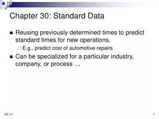
Chapter 30: Standard Data • Reusing previously determined times to predict standard times for new operations. • E.g., predict cost of automotive repairs • Can be specialized for a particular industry, company, or process …
Advantages of Using Standard Data • Cost • Time study is expensive. • Standard data allows you to use a table or an equation. • Ahead of Production • The operation does not have to be observed. • Allows estimates to be made for bids, method decisions, and scheduling. • Consistency • Values come from a bigger database. • Random errors tend to cancel over many studies. • Consistency is more important than accuracy.
Disadvantages of Standard Data • Imagining the Task • The analyst must be very familiar with the task. • Analysts may forget rarely done elements. • Database Cost • Developing the database costs money. • There are training and maintenance costs.
Motions vs. Elements • Decision is about level of detail. • MTM times are at motion level. • An element system has a collection of individual motions. • Elements can come from an analysis, time studies, curve fitting, or a combination.
Constant vs. Variable • Each element can be considered either constant or variable. • Constant elements either occur or don’t occur. • Constant elements tend to have large random error. • Variable elements depend on specifics of the situation. • Variable elements have smaller random error.
Developing the Standard • Plan the work. • Classify the data. • Group the elements. • Analyze the job. • Develop the standard.
Curve Fitting • To analyze experimental data: • Plot the data. • Guess several approximate curve shapes. • Use a computer to determine the constants for the shapes. • Select which equation you want to use.
Statistical Concepts • Least-squares equation • Standard error • Coefficient of variation • Coefficient of determination • Coefficient of correlation • Residual
Curve Shapes Y independent of X • Y = A • Determine that Y is independent of X by looking at the SE.
10 8 6 4 2 [y] y=4 0 2 4 6 8 10 [x] Y Independent of X • If Y is not related to X (is independent of X), then Y=A, where A is constant.
Curve Shapes Y depends on X, 1 variable • Y = A + BX • Y = AXB • Y = AeBX • Y = A + BXn • Y = X / (A + BX) • Y = A + BX + CX2
Curve Shapes Y depends on X, multiple variables • Y = A + BX + CZ • Results in a family of curves
Equations for Walking • NOTE: see attached Excel sheet intercept = ______ slope = _________ r2 = _______ σ = __________ • Therefore, Walk time is computed as: t = __________________ • So, if a new task is added that requires walking 7.4 m, how long should be allowed in the standard?
Equations for Walk Data Set Walk time h = –.13 + .11 (loge Distance, m) r2 = .966 σ = .012 h 1/Walk time h = .24 – .96 (1/Distance, m) r2 = .881 σ = .021 h-1