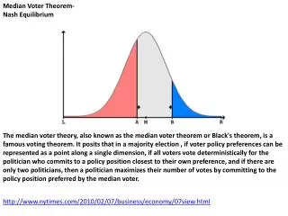
Computing Nash Equilibrium

Computing Nash Equilibrium Presenter: Yishay Mansour

Outline • Problem Definition • Notation • Today: Zero-Sum game • Next week: General Sum Games • Multiple players

Model • Multiple players N={1, ... , n} • Strategy set • Player i has m actions Si = {si1, ... , sim} • Siare pure actions of player i • S = i Si • Payoff functions • Player i ui : S  

Strategies • Pure strategies: actions • Mixed strategy • Player i – pi distribution over Si • Game - P = i pi • Product distribution • Modified distribution • P-i = probability P except for player i • (q, P-i ) = player i plays q other player pj

Notations • Average Payoff • Player i: ui(P) = Es~P[ui(s)] =  P(s)ui(s) • P(s) = i pi (si) • Nash Equilibrium • P* is a Nash Eq. If for every player i • For any distribution qi • ui(qi,P*-i)  ui(P*) • Best Response

Notations • Alternative payoff • xij(P) = ui(sij,P-i) = Es~P[ui(s) | si = sij] • Difference in payoff • zij(P) = xij(P) – ui(P) • Improvement in payoff • gij(P) = max{ zij(P),0}

Fixed point Theorems • Intermediate Value Theorem • domain [a,b] • function f continuous • f(a) f(b) < 0 • exists z such that f(z)=0 • Proof: M+ = { x | f(x) 0} M- ={x | f(x)  0} • closed sets and have an intersection.

Brouwer’s Fixed point theorem • f: S  S continuous, S compact and convex • There exists z in S : z = f(z) • For S=[0,1], previous theorem

Kakutani’ Fixed Point Theorem • L: S  S correspondence • L(x) is a convex set • L semi-continuous • S compact and convex • There exists z: z in L(z)

Nash Equilibrium I • Best response correspondence • L(P) = argmaxQ { ui(qi, P-i)} • L is a correspondence, continuous • Nash is a fixed point of L • P* in L(P*) • Kakutani’s fixed point theorem

Nash Equilibrium II • Fixed point • K(P) has mN parameters • Kij(P) = (pij+gij(P)) / (1 +  gij(P)) • Nash is a fixed point of K • P* = K(P*) • Original proof of Nash • Continuous function on a compact space • Brouwer’s fixed point theorem

Nash Equilibrium III • Non-linear complementary problem (NCP) • Recall zij(P) • For every player i and action aij: • zij(P)*pij = 0 • zi(P) is orthogonal to pi • Nash: z(P*)  0 • zij(P*)  0

Nash Equilibrium IV • Stationary point problem • Recall: x = alternative payoff • Nash: P* • For every P • (P-P*) x(P*)  0 • (pij –p*ij) x(P*)  0

Nash Equilibrium V • Minimizing a function • Objective function: • V(P) = i j [gij(P)]2 • V(P) is continuous and differentiable, non-negative function • NASH: V(P*) = 0 • Local Minima

Nash Equilibrium VI • Semi-Algebraic set • distribution P: j pij = 1 • difference in payoff: • zij(P)  0 • zij(P) = xij(P) – ui(P)  0 • Explicitly:

Two player games • Payoff matrices (A,B) • m rows and n columns • player 1 has m action, player 2 has n actions • strategies p and q • Payoffs: u1(pq)=pAqtand u2(pq)= pBqt • Zero sum game • A= -B

Linear Programming • Primal LP: • x in SETprimal is feasible • maximize <c,x> subject to x in SETprimal

Linear Programming • Dual LP: • y in SETdual is feasible • minimize <b,y> subject to y in SETdual

Duality Theorem • Weak duality: <c,x>  <b,y> • for any feasible x and y • proof! • Strong Duality • If there are feasible solutions then • <c,x> = <b,y> for some feasible x and y • sketch of proof.

Two players zero sum • Fix strategy q of player 2, • player 1 best response: • maximize p (Aqt) such that j pj = 1 and pj 0 • dual LP: minimize u such that u  Aqt • Player 2: select strategy q : • minimize u such that u  Aqtand i qi = 1 and qi 0 • dual (strategy for player 1) • maximize v such that v  pA, j pj = 1 and pj 0 • There exists a unique value v.

Example

Summary • Two players zero sum • linear programming • polynomial time • can have multiple Nash • unique value! • If (p,q) and (p’,q’) Nash then • (p,q’) and (p’,q) Nash

Online learning • Playing with unknown payoff matrix • Online algorithm: • at each step selects an action. • can be stochastic or fractional • Observes all possible payoffs • Updates its parameters • Goal: Achieve the value of the game • Payoff matrix of the “game” define at the end

Online learning - Algorithm • Notations: • Opponent distribution Qt • Our distribution Pt • Observed cost M(i, Qt) • Should be MQt • Goal: minimize cost • Algorithm: Exponential weights • Action i has weight proportional to bL(i,t) • L(i,t) = loss of action i until time t

Online algorithm: Notations • Formally: • parameter: b 0< b < 1 • wt+1(i) = wt(i) bM(i,Qt) • Zt =  wt(i) • Pt+1(i) = wt+1(i) / Zt • Number of total steps T is known

Online algorithm: Theorem • Theorem • For any matrix M with entries in [0,1] • Any sequence of dist. Q1 ... QT • The algorithm generates P1, ... , PT • RE(A||B) = Ex~A [ln (A(x) / B(x) ) ]

Online algorithm: Analysis • Lemma • For any mixed strategy P • Corollary

Online Algorithm: Optimization • b= 1/(1 + sqrt{2 (ln n) / T}) • Average Loss: v + O(sqrt{(ln n )/T})

Two players General sum games • Input matrices (A,B) • No unique value • Computational issues: find some, all Nash • player 1 best response: • Like for zero sum: • Fix strategy q of player 2 • maximize p (Aqt) such that j pj = 1 and pj 0 • dual LP: minimize u such that u  Aqt

Two players General sum games • Assume the support of strategies known. • p has support Sp and q has support Sq • Can formulate the Nash as LP:

Approximate Nash

Lemke & Howson

Example

Computing Nash Equilibrium