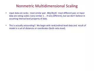
Nonmetric Multidimensional Scaling (NMDS)

Nonmetric Multidimensional Scaling(NMDS)

Nonmetric Multidimensional Scaling(NMDS) • Developed by Shepard (1962) and Kruskal (1964) for psychological data • First applied in ecology by Anderson (1971) • Based on a fundamentally different approach than the eigenanalysis methods PCA, CA (and DCA) • Axes of NMDS are not rotated axes of a high-dimensional “species space”.

The model of NMDS • NMDS works in a space with a specified number (small) of dimensions (e.g., 2 or 3) • The objects on interest (usually SUs in ecological applications) are points in this ordination space • The data on which NMDS operates are in the dissimilarity matrix among all pairs of objects (e.g., Bray-Curtis dissimilarities computed from community data).

The model of NMDS • NMDS seeks an ordination in which the distances between all pairs of SUs are, as far as possible, in rank-order agreement with their dissimilarities in species composition.

SU 4 SU 2 SU 1 Axis 2 SU 3 SU 5 Axis 1

Model of NMDS • Let Dij be the dissimilarity between SUs i and j, computed with any suitable measure (e.g. Bray-Curtis) • let ij be the Euclidean distance between SUs i and j in the ordination space.

Model of NMDS • The objective is to produce an ordination such that:Dij < Dkl ij  kl for all i, j, k, l • if any given pair of SUs have a dissimilarity less than some other pair, then the first pair should be no further apart in the ordination than the second pair • a scatter plot of ordination distances, ,against dissimilarities, D, is known as a Shepard diagram.

Shepard Diagram Distance,  Dissimilarity, D

Model of NMDS • The degree to which distances agree in rank-order with dissimilarities can be determined by fitting a monotone regression of the ordination distances  onto the dissimilarities D • A monotone regression line looks like an ascending staircase: it uses only the ranks of the dissimilarities • The fitted values, , represent hypothetical distances that would be in perfect rank-order with the dissimilarities.

Shepard Diagram with Monotone Regression  Distance,  Distance,  Dissimilarity, D Dissimilarity, D

Badness-of-fit: “Stress” • The badness-of-fit of the regression is measured by Kruskal’s stress, computed as: Residual sum ofsquares of monotone regression Sum ofsquares of distances

Contributions to Stress (Badness-of-fit) Distance,  Dissimilarity, D

Model of NMDS • Stress decreases as the rank-order agreement between distances and dissimilarities improves • The aim is therefore to find the ordination with the lowest possible stress • There is no algebraic solution to find the best ordination: it must be sought by an iterative search or trial-and-error optimization process.

Basic Algorithm for NMDS • Compute dissimilarities, D, among the n SUs using a suitable choice of data standardization and dissimilarity measure • Specify the number of ordination dimensions to be used • Generate an initial ordination of the SUs (starting configuration) with this number of axes • This can be totally random or an ordination of the SUs by some other method might be used.

Basic Algorithm for NMDS • Calculate the distances, , between each pair of SUs in the current ordination • Perform a monotone regression of the distances, , on dissimilarities, D • Calculate the stress • Move each SU point slightly, in a manner deemed likely to decrease the stress • Repeat steps 4 – 7 until the stress either approaches zero or stops decreasing (each cycle is called an iteration).

Basic Algorithm for NMDS • Any suitable optimization method can be used at step 7 to decide how to move each point • Stress can be considered a function with many independent variables: the coordinates of each SU on each axis • The aim is to find the coordinates that will minimize this function • This is a difficult problem to solve, especially when n is large.

Local Optima • There is no guarantee that the ordination with the lowest possible stress (global optimum) will be found from any given initial ordination • The search may arrive at a local optimum, where no small change in any coordinates will make stress decrease, even though a solution with lower stress does exist.

Local Optima Stress Local Optimum Global Optimum

Local Optima • run the entire ordination from several different starting configurations (typically at least 100) • if the algorithm converges to the same minimum stress solution from several different random starts, one can be confident the global optimum has been found.

Worked Example of NMDS • Densities (km-1) of 7 large mammal species in 9 areas of Rweonzori National Park, Uganda.

Worked Example of NMDS • Bray-Curtis dissimilarity matrix among the 9 areas. • Really only need the lower triangle, without the zero diagonals.

Initial Ordination (Random)

Initial Shepard Diagram

Stress • stress of initial (random) ordination is 0.4183 • This is high, reflecting the poor rank-order agreement of distances with dissimilarities at this stage. • each SU point is now moved slightly

How the ordination evolved Axis 2 Axis 1

How stress changed Stress Iteration Number

Shepard Diagram – Iteration 5

How the ordination evolved Axis 2 Axis 1

The Journey of Area 3 Start Final Axis 2 10 5 20 Axis 1

How stress changed Stress Once stress starts to level out, most SUs don’t change much in their position Iteration Number

Final NMDS Ordination Stress = 0.0139

Dimensionality • There is no way of knowing in advance how many dimensions you need for a given data set • To determine how many dimensions are needed, NMDS must be run in a range of dimensionalities • The vast majority of community data sets can be adequately summarized with 2 or 3 NMDS axes; rarely 4 or 5 may be needed.

Dimensionality • no simple relationship between axes in NMDS solutions for different numbers of dimensions • e.g. axes 1 and 2 of a 3-D NMDS are not the same as axes 1 and 2 of the 2-D solution • always possible to achieve a lower stress with an increase in dimensionality

Scree Plots • A line plot of minimum stress (Y axis) against number of dimensions is called a scree plot • It can be used as a guide in deciding on the number of dimensions required • A sharp break in slope of the curve, beyond which further reductions in stress are small, suggests dimensionality.

Scree Plot

Scree Plots • only a rough guide • sharpness of the “break” in slope depends on the “signal to noise ratio” of the data • the scree plot should be used to estimate the minimum number of axes required • If scree plot suggests k axes, also save and examine the k+1 dimensional solution.

Scree Plot

How low is low? • Kruskal and later authors suggest guidelines for interpreting the stress values in NMDS • NMDS ordinations with stresses up to 0.20 can be ecologically interpretable and useful.

Recommended Strategy for Choosing Number of Dimensions • use scree plot as a guide to minimum number of dimensions needed • if scree plot suggests k, save k-dimensional and (k+1)-dimensional solutions • interpret k-dimensional ordination • patterns of community change • correlations with environmental or other explanatory variables • then see if the extra axis of the (k+1)-D ordination adds interpretable information.

“Unstable” Solutions & PCORD • Trials with PCORD suggest that its algorithm for NMDS is much more prone to being trapped at local optima than other programs (e.g. SAS, DECODA) • The best way to avoid “unstable” solutions is not to use PCORD for NMDS.

Evaluation of NMDS Performance • Minchin (1987) compared of NMDS with other ordination methods (PCA, DCA) using simulated data • Model properties varied included: • Shape of response curves (symmetric, skewed, monotonic) • Beta diversity of gradients • Sampling pattern in “gradient space” • Amount of random variation (“noise”).

Simulated Gradient Space(Target “Ideal” Ordination Result) Gradient 2 Gradient 1

NMDS=0.13 DCA=0.09 CA=0.10

NMDS=0.08 DCA=0.19 CA=0.16

NMDS=0.08 DCA=0.19 CA=0.29

DCA=0.34 NMDS=0.09 CA=0.29

Nonmetric Multidimensional Scaling (NMDS)