
Lecture 2
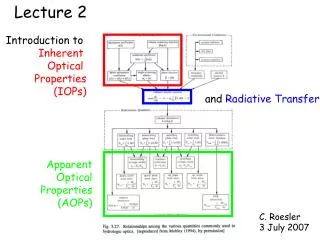
Introduction to Inherent Optical Properties (IOPs). and Radiative Transfer. Apparent Optical Properties (AOPs). Lecture 2. C. Roesler 3 July 2007. Readings. Mobley (Light and Water) section 1.4 Solid Angles section 3.1 IOPs section 3.2 AOPs section 5.10 Divergence Law.

Lecture 2
E N D
Presentation Transcript
Introduction to Inherent Optical Properties (IOPs) and Radiative Transfer Apparent Optical Properties (AOPs) Lecture 2 C. Roesler 3 July 2007
Readings • Mobley (Light and Water) • section 1.4 Solid Angles • section 3.1 IOPs • section 3.2 AOPs • section 5.10 Divergence Law
Inherent Optical Properties • inherent to the water • dependent upon the composition and concentrations of the particulate and dissolved substances and the water itself • independent of external properties such as the light field (i.e. should be the same if measured in situ or in discrete sample)
What are the IOPs? • Absorption, a • Color • Darkens • Scattering, b • Clarity • Brightens
What are the IOPs? • Absorption, a • Scattering, b • Beam attenuation, c (transmission) a + b = c The IOPs tell us something (e.g. concentration, composition) about the particulate and dissolved substances in the aquatic medium; how we measure them determines what we can resolve
Fo Ft Incident Radiant Flux Transmitted Radiant Flux Review of IOP Theory No attenuation
Conservation of radiant flux Fb Scattered Radiant Flux Fa Absorbed Radiant Flux Fo Ft Transmitted Radiant Flux Incident Radiant Flux Fo =
Beam Attenuation Theory Attenuance C = fraction of incident radiant flux attenuated Fb Fa Fo Ft • C = • C =
0c dx = x x Beam Attenuation Theory c = fractional attenuance per unit distance • c = Fb • c Dx = Fa Fo Ft • c(x-0) = • c x = • c x = • c (m-1) = Dx
Beam Attenuation: The Measurement Reality • c = (-1/x)ln(Ft/Fo) source detector Fa Fb Ft Fo x Detected flux (Ft) measurement must excludescattered flux
Beam Attenuation The Measurement Reality • c = (-1/x)ln(Ft/Fo) The size of the detector acceptance angle (FOV) determines the retrieved value of c source Fa Fb Ft Fo x The larger the detector acceptance angle,
Ex. transmissometer/c-meter Roesler and Boss 2004 FOV % b detected 0.018o <1 0.7o ~ 5 0.86o ~ 7 1.5o ~14 1.9o ~18
Absorption Theory a = fractional absorptance per unit distance • A = Fb • A = Fa • a = Fo Ft • a (m-1) = need to measure Dx
detector diffuser undetected scattered flux must be corrected for Absorption Measurement Reality • a = (-1/x)ln[(Ft + Fb)/Fo] Detected flux measurement must include scattered flux source Fa Fb Fo Ft x
Currently the only commercially available absorption meter: WETLabs ac9
AC9 25 cm absorption tube optimized to collect scattered flux attenuation tube optimized to reject scattered flux
How much scattered light is detected? Theoretically • Detector FOV ~ 40o • ~90% of scattered flux • 10% of scatter can ~abs • loss is in side and backward directions • must correct for scattering losses
Scattering, b, has an angular dependence, which is described by the volume scattering function, b(q, f) = power per unit steradian emanating from a volume illuminated by irradiance = dF1 1 dW dV E dV = dS dr E = F/dS [mmol photon m-2 s-1] dr E ↑ dS = 1 dF FodrdW b(q,f) =dF1 dS dW dSdr Fo And b = ∫4p b(q,f) dW sinq dq df What is dW?
So we can calculate scattering, b, from the volume scattering function,b(q,f) = ∫ 0∫0 b(q,f) sinq dq df 2p p If there is azimuthal symmetry = 2p∫0 b(q,f) sinq dq p p bf = 2p∫0 b(q,f) sinq dq and bb = 2p∫p/2 b(q,f) sinq dq p/2 ~ We define the phase function: b(q,f) = b(q,f) b b = ∫4p b(q,f) dW
Ft Fo Fo r Summary of the IOPs Note: c = a + b w is not solid angle in this case w≡ b/c single scattering albedo is related toa, r if 1) all scattered light detected 2) optical path = geometric path is related toc, r if 1) no scattered light detected Then b = c - a
Apparent Optical Properties Derived from radiometric parameters Depend upon the light field Depend upon the IOPs Ratios or gradients of radiometric parameters “Easy” to measure Difficult to interpret
Apparent Optical Properties What is the color and brightness of the ocean? How does sunlight penetrate the ocean? How does the angular distribution of light vary in the ocean?
md = mu = Eu. Eou m = Ed - Eu. Eo AOPs: Average Cosines L (q,f) [mmol photons m-2 s-1 sr-1] Ed = ∫02p∫0p/2L (q,f) cosq dW Eod = ∫02p∫0p/2L (q,f) dW Ratios of radiometric parameters
md = Ed = ∫02p∫0p/2L (q,f) cosq sinq dq df Eod∫02p∫0p/2L (q,f) sinq dq df md = in terms of degrees q = average cosines are not unique quantities Example of isotropic light field • L(q,f) constant for all q,f and then the math happens… (i.e. you try it!)
AOPs: Reflectance L (q,f) [mmol photons m-2 s-1 sr-1] Ed = ∫02p∫0p/2L (q,f) cosq dW Eod = ∫02p∫0p/2L (q,f) dW Ratios of radiometric parameters R = Eu. Irradiance Ed Reflectance RRS = Lu. Remote Sensing or Ed Radiance Reflectance
0.01 0.012 0.04 0.02 0.006 0.03 0.09 0.015 Roesler et al 2003 Roesler and Perry 1995 Reflectance Ranges
E z AOPs: diffuse attenuation coefficients L (q,f) [mmol photons m-2 s-1 sr-1] Ed = ∫02p∫0p/2L (q,f) cosq dW Eod = ∫02p∫0p/2L (q,f) dW Radiometric Gradients dE(z) = -K(z) E(z) dz K(z) dz = -1 dE E(z) ∫z if K was constant with z K z = -ln(E(zo)) + ln(E(z)) K = -1 ln(E(zo)/E(z)) z E(z) = E(zo) e-Kz
AOPs: diffuse attenuation coefficients Why would K vary with depth? generated from HL by Curt Zaneveld et al. 2001 Opt Exp
Ed1Ed2 constant c z Kd1Kd2 AOPs: diffuse attenuation coefficients NOTE c K c beam attenuation K diffuse attenuation <
dz = absorption along path r scattering out of path r scattering into path r Radiative Transfer Equation Consider the radiance, L(q,f), as it varies along a path r through the ocean, at a depth of z d L(q,f), what processes affect it? dr
Radiative Transfer Equation Consider the radiance, L(q,f), as it varies along a path r through the ocean, at a depth of z d L(q,f), what processes affect it? dr cosq d L(q,f) = -a L(z,q,f) -b L(z,q,f) + ∫4pb(z,q,f;q’,f’)L(q’,f’)dW’ dz If there are sources of light (e.g. fluorescence, raman scattering, bioluminescence), that is included too: a(l1,z) L(l1,z,q’,f’) →(quantum efficiency) → L(l2,z,q,f)
d(Ed – Eu) = dz An example of the utility of RTE cosq d L(q,f) = -a L(z,q,f) -b L(z,q,f) + ∫4pb(z,q,f;q’,f’)L(q’,f’)dW’ dz Divergence Law (see Mobley 5.10) Integrate the equation over all solid angles (4 p), dW 0∫2p0∫pd L(q,f) cosq sin q dq df = dz 0∫2p0∫p -c L(z,q,f) sin q dq df= 0∫2p0∫p[0∫2p 0∫pb(z,q,f;q’,f’) L(q’,f’) sin q dq’df’] sin q dq df = [0∫2p 0∫pb(z,q,f;q’,f’) sin q dq df] 0∫2p0∫p[0∫2p 0∫pb(z,q,f;q’,f’) sin q dq df] L(q’,f’) sin q dq’df’ = dĒ = dz
divide both sides by E a = KĒmGershun’s Equation KĒ = a . m An example of the utility of RTE cosq d L(q,f) = -a L(z,q,f) -b L(z,q,f) + ∫4pb(z,q,f;q’,f’)L(q’,f’)dW’ dz . . . dĒ = -c Eo + b Eo dz -1 dĒ = a Eo Ē dz Ē substitute AOPs
Readings for Lecture 3 (Absorption) • Mobley • section 3.3 Optically significant constituents • section 3.7 Absorption


