Search Algorithms for Agents

CISC 886: MultiAgent Systems Fall 2004 Search Algorithms for Agents Sachin Kamboj

Outline • Introduction • Path-Finding Problems • Formal Definition • Asynchronous Dynamic Programming • Learning Real Time A* • Moving Target Search • Real –Time Bidirectional Search • Constraint Satisfaction Problems • Formal Definition • Filtering Algorithm • Hyper-Resolution Based Consistency Algorithm • Asynchronous Backtracking • Distributed Constraint Optimization Problems • Adopt (Asynchronous Distributed Optimization) • OptAPO (OPTimal Asynchronous Partial Overlay)

Introduction • Search: • an umbrella term for various problem solving techniques in AI • used when the sequence of actions required for solving a problem is not known a priori • hence trial and error exploration of the alternatives is required • Search algorithms are designed to solve three classes of problems: • Path-finding problems • Constraint satisfaction problems • Competitive games

Introduction • A whole set of search algorithms exist for single agents • have known properties (like time and space complexity). • have been used effectively to solve a large number of AI problems. • Examples: BFS, DFS, Branch and Bound, A* • So, why use multiple agents? • Agents have limited rationality • search is often intractable • may not have a complete picture of the problem • may not have the required computational capability • Agents may be self interested

Agent 2 Agent 3 Agent 1 Introduction • Approach • If we represent the search problem as a graph, we can solve it by accumulating local computations for each node in the graph. • Local computations can be executed asynchronously and concurrently

Introduction • Advantages of asynchronous search algorithms: • Local computations needed will fit within the limited rationality of the agents • Execution order of these algorithms can be highly flexible and arbitrary

Path Finding Problems

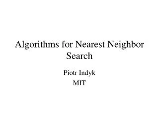
Goal Start Example 1: Finding a path through a Maze

1 1 1 4 4 1 4 4 2 2 2 2 2 3 3 6 1 3 3 3 3 4 5 5 5 5 5 6 6 6 6 7 7 7 7 7 8 8 8 8 8 Initial State Goal State Example 2: Solving the 8-puzzle problem

Formal Definition • A path finding problem consists of the following components: • A set of nodes, N, each representing a state • A set of directed links, L, each representing an operator available to a problem solving agent • A unique start state, S • A set of goal states, G • A set of weights, W, associated with each link • represent the cost of applying the operator • called the “distance” between the nodes • Neighbors are nodes that have directed links between them

Principle of Optimality • States that a path is optimal if and only if every segment of it is optimal

Asynchronous Dynamic Programming • Let: • h*(i) = shortest distance from node i to the goal • k(i,j) = cost of link between i and j • f*(j) = shortest distance from node i to goal via a neighboring node j f*(j) = k(i,j) +h*(j) • By the principle of optimality: h*(i) = minj f*(j) • Asynchronous dynamic programming computes h* by repeating the local computations of each node

Asynchronous Dynamic Programming • Assumes the following situation: • For each node, i, there exists a process corresponding to i • Each process records h(i), which is the estimated value of h*(i). • The initial value of h*(i) is arbitrary (e.g., , 0) except for the goal nodes • For each goal node g, h(g) is 0. • Each process can refer to h values of neighboring nodes (via shared memory or message passing)

Asynchronous Dynamic Programming • Each process updated h(i) by the following procedure: • For each neighboring node j: • Compute f(j) = k(i,j) + h(j) where • h(j) is the current estimated distance from j to a goal node • k(i,j) is the cost of the link from i to j • update h(i) as follows • h(i) ← minj f(j)

2 1 1 1 1 1 3 3 2 Asynchronous Dynamic Programming • Example: 3 1    0 initial state goal state  2  2 3

Asynchronous Dynamic Programming • Is the algorithm complete? • Yes • Is the algorithm optimal? • Yes • Are there any problems? • cannot be used for reasonably large path-finding problems • we cannot afford to have processes for all the nodes

Learning Real-Time A* • Used when: • only one agent is present • not possible to perform local computations for all nodes • when planning and execution needs to be interleaved • In this algorithm: • the agents selectively execute the computations for the current node • each agent repeats the following procedure: • Lookahead: calculate f(j) = k(i,j) + h(j) • Update: the estimate of node i as h(i) ← minj f(j) • Action Selection: Move to the neighbor j that has the minimum f(j) value. Ties are broken randomly

Learning Real-Time A* • Requirement: • the initial value of h must be optimistic, i.e. h(i)  h*(i) • Is the algorithm complete? • Yes, in a finite number of nodes with positive link costs, in which there exists a path from every node to a goal node, and starting with non-negative initial estimates, LRTA* will eventually reach a goal node • Is the algorithm optimal? • Requires repeated trials for optimality • If the initial estimates are admissible, then over repeated problem solving trials, the values learned by LRTA* will eventually converge to their actual distances along every optimal path to the goal node

Moving Target Search • Allows the goal state to change during the course of the search • For example, a robot’s task is to reach another robot which is in fact moving as well • The target robot may • cooperatively try to reach the problem solving robot • actively avoid the problem solving robot • move independent of the problem solving robot • In order to guarantee success, the problem solver must be able to move faster than the target

Moving Target Search • Is a generalization of LRTA* • The algorithm: • does NOT maintain a single heuristic of the distance to the target goal • instead tries to acquire heuristic information for each potential target location. • Thus, MTS maintains a matrix of heuristic values, representing the function h(x,y) for all pairs of states x and y • The matrix is updated on each move of the problem solver and the target.

Moving Target Search • Let xi and xj be the current and neighboring positions of the problem solver and yi and yj be the current and neighboring positions of the target. • Assume all edges in the graph have unit cost • When the problem solver moves: • Calculate h(xj,yi) for each neighbor xj of xi. • Update the value of h(xi,yi) as follows: h(xi,yi) ← max ( h(xi,yi) , minxj{h(xj,yi) + 1} ) • Move to the neighbor xj with the minimum h(xj,yi), i.e. assign the value of xj to xi. Ties are broken randomly.

Moving Target Search • When the problem solver moves: • Calculate h(xi,yj) for the target’s new position yj. • Update the value of h(xi,yi) as follows: h(xi,yi) ← max ( h(xi,yi) , h(xj,yj) – 1 ) • Reflect the target’s new position as the new goal of the problem solver, i.e. assign the value of yj to yi. • Is the algorithm complete? • Yes, A problem solver executing MTS is guaranteed to eventually reach the target • Is the algorithm optimal? • No

Real –Time Bidirectional Search • Two problem solvers starting from the initial and goal states physically move towards each other. • Planning and execution are interleaved • The following steps are repeatedly executed until the two problem solvers meet in the problem space: • Control Strategy: Select a forward (step2) or backward move (step3) • Forward Move: The problem solver starting from the initial stage (i.e. the forward problem solver) moves towards the problem solver starting from the goal state. • Backward Move: The problem solver starting from the goal stage (i.e. the backward problem solver) moves towards the problem solver starting from the initial state.

Real –Time Bidirectional Search • Can be classified into two categories: • Centralized RTBS • The best action is selected among all possible moves of the two problem solvers • The control strategy selects which of the two problem solvers to run depending on what the best action is • Two centralized RTBS algorithms (based on LRTA* and RTA*) can be implemented • Decoupled RTBS • The two problem solvers independently make their own decisions. • The control strategy alternatively runs the forward and backward problem solvers • MTS can be used for implementing decoupled RTBS.

Constraint Satisfaction Problems

Example 1: Scheduling a set of tasks • A set of exams need to be scheduled during the last week of December. No more than 5 exams can be scheduled on a Tuesday and no more than 7 exams on any other day………

X1 X2 { red, blue, yellow } { red, blue, yellow } { red, blue, yellow } X3 { red, blue, yellow } X4 Example 2: Graph-Coloring Problem • Objective: • To paint the nodes of a graph so that any two nodes connected by a link do not have the same color. • Each node has a finite number of possible colors

Formal Definition • A constraint satisfaction problem consists of: • A set of n variables V = {x1, x2, …, xn } • Discrete, finite domains for each of the variables D = { D1, D2, …, Dn } • A set of constraints on the value of the variables. • The constraints are defined by predicates, pk(xk1, xk2, …, xkj) where each pk is the function pk : Dk1 x Dk2 x … x Dkj {0 , 1}. • The problem is to find an assignment of values to the variables such that all the constraints are satisfied. • Constraint satisfaction is NP-complete in general • A trial and error exploration of alternatives is inevitable

Relation to DAI • We assume that the variables of the CSP are distributed amongst multiple agents. • Many application problems in DAI can be formalized as distributed constraint satisfaction problems. • For example: • interpretation problems • assignment problems, and • multiagent truth maintenance problems • For simplicity, we assume an agent for each variable in all the algorithms

Filtering Algorithm • Each agent communicates its domain to its neighbor and then removes values that cannot satisfy constraints from its domain. • More specifically, a process (agent), xi performs the following procedure revise(xi,xj) for each neighbor xj. procedurerevise (xi, xj) for all vi Dido if there is no value vj  Dj such that vj is consistent with vi then delete vi from Di; end if; end do; • If some value of the domain is removed by performing the procedure revise, process xi sends the new domain to its neighboring processes. • If a new domain is received from a neighbor, call procedure revise again.

X1 X2 { red, blue, yellow } { red } { blue } X3 { red, blue, yellow } X4 Filtering Algorithm • For example, • As a result of the filtering algorithm, x1 will remove red and blue from its domain and x4 will remove blue from its domain.

Filtering Algorithm • If the domain of some variable becomes the empty set: • the problem is over-constrained and has no solution • If each domain has a unique value: • the assignment of the unique values to the variables is a solution. • If there exist multiple values for some variable: • we cannot tell whether the problem has a solution or not • further trial and error search is required to find a solution • Filtering algorithms cannot solve CSP problems in general • This algorithm is used as a preprocessing procedure before the application of some other method.

X1 X2 { red, blue } { red, blue } { red, blue } X3 Hyper-Resolution Based Consistency Algorithm • All constraints are represented as a “nogood” • a prohibited combination of variable values. • For example, in the figure below: • A constraint between x1and x2 can be represented using two nogoods: • {x1 = red, x2 = red} • {x1 = blue, x2 = blue} • The algorithm uses several existing nogoods and the domain of a variable to generate a new nogood.

Hyper-Resolution Based Consistency Algorithm • For example, using the nogoods: • {x1 = red, x2 = red} • {x1 = blue, x3 = blue} and the domain of x1 {red, blue}, a new nogood: • {x2 = red, x3 = blue} is generated • The hyper-resolution rule is described as follows: A1 V A2 V … V Am  (A1  A11 … )  (A2  A21 … ) : :  (Am  Am1 … )  (A11  …  A21 …  Am1 …)

Asynchronous Backtracking • Asynchronous version of a backtracking algorithm • standard method for solving CSPs • Each variable/process is assigned a priority • usually based on the alphabetical order of the variable identifiers • Each process selects a random value from its domain • Each process communicates its tentative variable assignments to its neighboring processes. • If the current value of a process is not consistent with the assignment of higher priority processes, the process changes its value • If no consistent value exists, generate a new nogood and send it to the higher priority process • On receiving a nogood, higher priority process changes its value. • Each process maintains the current variable assignments of other processes in its local_view. • May contain obsolete information.

Asynchronous Backtracking • Two main types of messages are communicated: • ok? messages to communicate the current value • nogood messages to communicate a new nogood • Example: (nogood {(x1, 1) }) X1 X2 add neighbor request { 1, 2 } { 2 } local_view {(x1, 1) }   (ok? (x1, 1)) (ok? (x2, 2)) (nogood {(x1, 1), (x2, 2) }) { 1, 2 } X3 local_view {(x1, 1), (x2, 2) }

Distributed Constraint Optimization Problems • Are a generalization of constraint satisfaction problems • Like DCSP, DCOP includes a set of variables: • each variable is assigned to an agent that has control over its value • In DCSP • the agents assign values to variables so as to satisfy the constraints on them • In DCOP • the agents must coordinate their choice of values so that a global objective function is optimized. • Applications of DCOP: • Multiagent Teamwork • Distributed Scheduling • Distributed Sensor Networks

Distributed Constraint Optimization Problems • Formal Definition • A constraint satisfaction problem consists of: • A set of n variables V = {x1, x2, …, xn } • Discrete, finite domains for each of the variables D = { D1, D2, …, Dn } • A set of cost functions f = {f1, …, fm} . • where each fi is a function fi : Di1 x Di2 x … x Dij N U . • The problem is to find an assignment A* = {d1, …, dn | di  Di} such that the global cost called F, is minimized. • F is defined as follows:

Distributed Constraint Optimization Problems • Design Criteria for DCOP algorithms: • Agents should be able to optimize a global function in a distributed fashion using only local communication • The agents should operate asynchronously • agents should not sit idle waiting for a particular message from a particular agent • The algorithm should provide provable quality guarantees on system performance

Adopt (Asynchronous Distributed Optimization) • Generalization of Asynchronous Backtracking • with a bunch of performance tweaks. • Starts by assigning a priority to the agents based on a depth-first search tree • each node has a single parent and multiple children • parents have higher priority than the children • hence, does not require a linear priority ordering on the agents • Constraints are only allowed between a node and any of its ancestors and descendants • there can be no constraints between different subtrees of the DFS tree • not a restriction of the constraint network itself

x1 x2 x3 x4 Adopt (Asynchronous Distributed Optimization) • Example: x1 x2 x3 x4 Constraint Graph DFS Tree

Adopt (Asynchronous Distributed Optimization) • Algorithm begins by all agents choosing their values concurrently • The algorithm uses three types of messages: • VALUE Messages: • used to send the current selected value of the variable to the descendants below the node in the DFS tree • similar to ok? messages in ABT • THRESHOLD Messages: • are only sent by a parent to its immediate children • contain a single number which represents the backtrack threshold • COST Messages: • are a generalization of nogood messages in ABT • contain the current context (same as in ABT) and the lb and the ub.

Adopt (Asynchronous Distributed Optimization) • The algorithm calculates the local cost using the formula: where δ(di) is the local cost at xi when xi chooses d. • This formula is used to calculate the cost of a node only on the basis of the constraints that the node shares with its ancestors (NOT its children) • This is because the current context is built from the VALUE messages received by a node • The node (xi)also calculates LB and UB • The idea is that LB and UB are the lower and upper bounds on the cost seen so far for a subtrees rooted at xi.

Adopt (Asynchronous Distributed Optimization) • For a leaf node, • lb(di) = ub(di) = δ(di) • For any other node, • For all nodes: • Similar for UB • By keeping a track of LB and UB, the agent knows the current lower bound and upper bound on cost in the subtrees • The algorithm uses a threshold values to decide when to backtrack

OptAPO • OPTimal Asynchronous Partial Overlay • used to increase the efficiency of previous DCOP algorithms (eg adopt) • previous DCOP algorithms were based on a total separation of the agents knowledge during the problem solving process • is based on a partial centralization technique called cooperative mediation • allows the agents to extend and overlap the context that they use for making their local decisions

OptAPO • When an agent acts as a mediator, it • computes a solution to the overall problem • recommends value changes to the agents involved in the mediation session

Questions?

Search Algorithms for Agents