Communication Lower Bounds for Matrix Multiplication in Parallel Algorithms
This lecture explores the communication costs associated with algorithms, particularly focusing on matrix multiplication using both reduction and geometric embedding approaches. We discuss the different models and their associated costs, including bandwidth and latency in both sequential and parallel contexts. Specific techniques to prove communication lower bounds for classical O(n^3) algorithms, like Cholesky and LU decompositions, are highlighted through existing research. Key proofs and theorems are presented, emphasizing the importance of communication efficiency in computational algorithms.

Communication Lower Bounds for Matrix Multiplication in Parallel Algorithms
E N D
Presentation Transcript
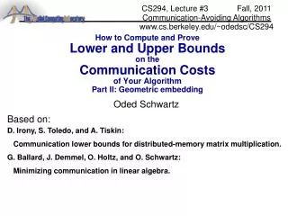
CS294, Lecture #3 Fall, 2011 Communication-Avoiding Algorithms www.cs.berkeley.edu/~odedsc/CS294 How to Compute and ProveLower and Upper Boundson theCommunication Costsof Your AlgorithmPart II: Geometric embedding Oded Schwartz Based on: D. Irony, S. Toledo, and A. Tiskin: Communication lower bounds for distributed-memory matrix multiplication. G. Ballard, J. Demmel, O. Holtz, and O. Schwartz: Minimizing communication in linear algebra.
Last time: the models Two kinds of costs: Arithmetic (FLOPs) Communication: moving data between levels of a memory hierarchy (sequential case) over a network connecting processors (parallel case) CPU Cache CPU RAM CPU RAM M1 M2 RAM M3 CPU RAM CPU RAM Mk = Parallel Sequential Hierarchy
Last time: Communication Lower Bounds Approaches: Reduction [Ballard, Demmel, Holtz, S. 2009] Geometric Embedding[Irony,Toledo,Tiskin 04],[Ballard, Demmel, Holtz, S. 2011a] Graph Analysis [Hong & Kung 81], [Ballard, Demmel, Holtz, S. 2011b] Proving that your algorithm/implementation is as good as it gets.
Last time: Lower bounds for matrix multiplication Bandwidth: [Hong & Kung 81] Sequential [Irony,Toledo,Tiskin 04] Sequential and parallel Latency: Divide by M.
Last time: Reduction (1st approach)[Ballard, Demmel, Holtz, S. 2009a] Thm: Cholesky and LU decompositions are(communication-wise) as hard as matrix-multiplication Proof: By a reduction (from matrix-multiplication) that preserves communication bandwidth, latency, and arithmetic. Cor: Any classical O(n3) algorithm for Cholesky and LU decomposition requires: Bandwidth: (n3 / M1/2) Latency: (n3 / M3/2) (similar cor. for the parallel model).
Today: Communication Lower Bounds Approaches: Reduction [Ballard, Demmel, Holtz, S. 2009] Geometric Embedding[Irony,Toledo,Tiskin 04],[Ballard, Demmel, Holtz, S. 2011a] Graph Analysis [Hong & Kung 81], [Ballard, Demmel, Holtz, S. 2011b] Proving that your algorithm/implementation is as good as it gets.
Lower bounds: for matrix multiplicationusing geometric embedding [Hong & Kung 81] Sequential [Irony,Toledo,Tiskin 04] Sequential and parallel Now: prove both, using the geometric embedding approach of [Irony,Toledo,Tiskin 04].
Geometric Embedding (2nd approach)[Irony,Toledo,Tiskin 04], based on [Loomis & Whitney 49] • Matrix multiplication form: • (i,j) n x n, C(i,j) = k A(i,k) B(k,j), Thm: If an algorithm agrees with this form (regardless of the order of computation) then BW = (n3/ M1/2) BW = (n3/ PM1/2) in P-parallel model.
For a given run (algorithm, machine, input) Partition computations into segmentsof M reads / writes Any segment S has 3M inputs/outputs. Show that #multiplications in S k The total communication BW isBW = BW of one segment #segments M #mults / k M Read S1 Read Read FLOP Write S2 FLOP Read Read Read FLOP Time FLOP S3 FLOP Write Write FLOP ... Geometric Embedding (2nd approach)[Irony,Toledo,Tiskin 04], based on [Loomis & Whitney 49] ... Example of a partition,M = 3
x y C B A z y z x C B A Geometric Embedding (2nd approach)[Irony,Toledo,Tiskin 04], based on [Loomis & Whitney 49] “C shadow” • Matrix multiplication form: • (i,j) n x n, C(i,j) = k A(i,k)B(k,j), “B shadow” “A shadow” V V Thm: (Loomis & Whitney, 1949) Volume of 3D set V ≤ (area(A shadow) · area(B shadow) · area(C shadow) ) 1/2 Volume of boxV = x·y·z = ( xz · zy · yx)1/2
For a given run (algorithm, machine, input) Partition computations into segmentsof M reads / writes Any segment S has 3M inputs/outputs. Show that #multiplications in S k The total communication BW isBW = BW of one segment #segments M #mults / k = M n3 / k By Loomis-Whitney:BW M n3 / (3M)3/2 M Read S1 Read Read FLOP Write S2 FLOP Read Read Read FLOP Time FLOP S3 FLOP Write Write FLOP ... Geometric Embedding (2nd approach)[Irony,Toledo,Tiskin 04], based on [Loomis & Whitney 49] ... Example of a partition,M = 3
From Sequential Lower bound to Parallel Lower Bound We showed: Any classical O(n3) algorithm for matrix multiplication on sequential model requires: Bandwidth: (n3 / M1/2) Latency: (n3 / M3/2) Cor: Any classical O(n3) algorithm for matrix multiplication on P-processors machine (with balanced workload) requires: 2D-layout: M=O(n2/P) Bandwidth: (n3 /PM1/2) (n2/P1/2) Latency: (n3 / PM3/2) (P1/2)
From Sequential Lower bound to Parallel Lower Bound Proof: Observe one processor. Is it always true? C B A “C shadow” “B shadow” “A shadow” Let Alg be an algorithm with communication lower bound B = B(n,M). Then any parallel implementation of Alg has a communication lower bound B’(n, M, p) = B(n, M)/p ?
Proof of Loomis-Whitney inequality z T(x=i | y) y T x x=i T(x=i) • T(x=i) = subset of T with x=i • T(x=i | y ) = projection of T(x=i) onto y=0 plane • N(x=i) = |T(x=i)| etc • N = i N(x=i) = i (N(x=i))1/2 · (N(x=i))1/2 • ≤ i (Nx)1/2 · (N(x=i))1/2 • ≤ (Nx)1/2 · i (N(x=i | y ) · N(x=i | z ))1/2 • = (Nx)1/2 · i (N(x=i | y ) )1/2 · (N(x=i | z ))1/2 • ≤ (Nx)1/2 · (i N(x=i | y ) )1/2 · (i N(x=i | z ))1/2 • = (Nx)1/2 · (Ny)1/2 · (Nz)1/2 N(x=i) N(x=i|y)·N(x=i|z) T(x=i) N(x=i|z) N(x=i|y) T = 3D set of 1x1x1 cubes on lattice N = |T| = #cubes Tx = projection of T onto x=0 plane Nx = |Tx| = #squares in Tx, same for Ty, Ny, etc Goal: N ≤ (Nx · Ny · Nz)1/2
Communication Lower Bounds Approaches: Reduction [Ballard, Demmel, Holtz, S. 2009] Geometric Embedding[Irony,Toledo,Tiskin 04],[Ballard, Demmel, Holtz, S. 2011a] Graph Analysis [Hong & Kung 81], [Ballard, Demmel, Holtz, S. 2011b] Proving that your algorithm/implementation is as good as it gets.
How to generalize this lower bound • Matrix multiplication form: • (i,j) n x n, C(i,j) = k A(i,k)B(k,j), (1) Generalized form: (i,j) S, C(i,j) = fij( gi,j,k1 (A(i,k1), B(k1,j)), gi,j,k2 (A(i,k2), B(k2,j)), …, k1,k2,… Sij other arguments) • C(i,j) any unique memory location.Same for A(i,k) and B(k,j). A,B and C may overlap. • Lower bound for all reorderings. Incorrect ones too. • It does assume each operand generate load/store. • Turns out QR, eig, SVD all may do this • Need a different analysis. Not today… • fij and gijk are “nontrivial” functions
Geometric Embedding (2nd approach) (1) Generalized form: (i,j) S, C(i,j) = fij( gi,j,k1 (A(i,k1), B(k1,j)), gi,j,k2 (A(i,k2), B(k2,j)), …, k1,k2,… Sij other arguments) Thm: [Ballard, Demmel, Holtz, S. 2011a] If an algorithm agrees with the generalized form then BW = (G/ M1/2) where G = |{g(i,j,k) | (i,j) S, k Sij} BW = (G/ PM1/2) in P-parallel model.
Example: Application to Cholesky decomposition (1) Generalized form: (i,j) S, C(i,j) = fij( gi,j,k1 (A(i,k1), B(k1,j)), gi,j,k2 (A(i,k2), B(k2,j)), …, k1,k2,… Sij other arguments)
From Sequential Lower bound to Parallel Lower Bound We showed: Any algorithm that agrees with Form (1) on sequential model requires: Bandwidth: (G/ M1/2) Latency: (G/ M3/2)where G is the gijk count. Cor: Any algorithm that agrees with Form (1), on a P-processors machine, where at least two processors perform (1/P) of G each requires: Bandwidth: (G/PM1/2) Latency: (G/ PM3/2)
Geometric Embedding (2nd approach)[Ballard, Demmel, Holtz, S. 2011a]Follows [Irony,Toledo,Tiskin 04], based on [Loomis & Whitney 49] Lower bounds: for algorithms with “flavor” of 3 nested loopsBLAS, LU, Cholesky, LDLT, and QR factorizations, eigenvalues and SVD, i.e., essentially all direct methods of linear algebra. Dense or sparse matrices In sparse cases: bandwidth is a function NNZ. Bandwidth and latency. Sequential, hierarchical, and parallel – distributed and shared memory models. Compositions of linear algebra operations. Certain graph optimization problems [Demmel, Pearson, Poloni, Van Loan, 11], [Ballard, Demmel, S. 11] Tensor contraction For dense:
Do conventional dense algorithms as implemented in • LAPACK and ScaLAPACK attain these bounds? • Mostly not. • Are there other algorithms that do? • Mostly yes.
Dense 2D parallel algorithms • Assume nxn matrices on P processors, memory per processor = O(n2 / P) • ScaLAPACK assumes best block size b chosen • Many references (see reports), Blueare new • Recall lower bounds: • #words_moved = ( n2 / P1/2 ) and #messages = ( P1/2 ) Relax: 2.5D AlgorithmsSolomonik & Demmel ‘11
For a given run (algorithm, machine, input) Partition computations into segmentsof M reads / writes Any segment S has 3M inputs/outputs. Show that S performs k FLOPs gijk The total communication BW isBW = BW of one segment #segments M G / k, where G is #gi,j,k M Read S1 Read Read FLOP Write S2 FLOP Read Read Read FLOP Time FLOP S3 FLOP Write Write FLOP ... Geometric Embedding (2nd approach) ... Example of a partition,M = 3
x y C B A z y z x C B A Geometric Embedding (2nd approach)[Ballard, Demmel, Holtz, S. 2011a]Follows [Irony,Toledo,Tiskin 04], based on [Loomis & Whitney 49] “C shadow” (1) Generalized form: (i,j) S, C(i,j) = fij( gi,j,k1 (A(i,k1), B(k1,j)), gi,j,k2 (A(i,k2), B(k2,j)), …, k1,k2,… Sij other arguments) V V “B shadow” “A shadow” Thm: (Loomis & Whitney, 1949) Volume of 3D set V ≤ (area(A shadow) · area(B shadow) · area(C shadow) ) 1/2 Volume of boxV = x·y·z = ( xz · zy · yx)1/2
For a given run (algorithm, machine, input) Partition computations into segmentsof M reads / writes Any segment S has 3M inputs/outputs. Show that S performs k FLOPs gijk The total communication BW isBW = BW of one segment #segments M G / k where G is #gi,j,k By Loomis-Whitney:BW M G / (3M)3/2 M Read S1 Read Read FLOP Write S2 FLOP Read Read Read FLOP Time FLOP S3 FLOP Write Write FLOP ... Geometric Embedding (2nd approach) ... Example of a partition,M = 3
Applications (1) Generalized form: (i,j) S, C(i,j) = fij( gi,j,k1 (A(i,k1), B(k1,j)), gi,j,k2 (A(i,k2), B(k2,j)), …, k1,k2,… Sij other arguments) BW = (G/ M1/2) where G = |{g(i,j,k) | (i,j) S, k Sij} BW = (G/ PM1/2) in P-parallel model. 27
Geometric Embedding (2nd approach)[Ballard, Demmel, Holtz, S. 2011a]Follows [Irony,Toledo,Tiskin 04], based on [Loomis & Whitney 49] (1) Generalized form: (i,j) S, C(i,j) = fij( gi,j,k1 (A(i,k1), B(k1,j)), gi,j,k2 (A(i,k2), B(k2,j)), …, k1,k2,… Sij other arguments) But many algorithms just don’t fit the generalized form! For example: Strassen’s fast matrix multiplication
Beyond 3-nested loops How about the communication costs of algorithms that have a more complex structure?
Communication Lower Bounds – to be continued… Approaches: Reduction [Ballard, Demmel, Holtz, S. 2009] Geometric Embedding[Irony,Toledo,Tiskin 04],[Ballard, Demmel, Holtz, S. 2011a] Graph Analysis [Hong & Kung 81], [Ballard, Demmel, Holtz, S. 2011b] Proving that your algorithm/implementation is as good as it gets.
Further reduction techniques: Imposing reads and writes Example: Computing ||A∙B|| where each matrix element is a formulas, computed only once. Problem: Input/output do not agree with Form (1). Solution: Impose writes/reads of (computed) entries of A and B. Impose writes of the entries of C. The new algorithm has lower bound For the original algorithm i.e., for (which we assume anyway). (1) Generalized form: (i,j) S, C(i,j) = fij( gi,j,k1 (A(i,k1), B(k1,j)), gi,j,k2 (A(i,k2), B(k2,j)), …, k1,k2,… Sij other arguments)
Further reduction techniques: Imposing reads and writes The previous example can be generalized to other “black-box” uses of algorithms that fit Form (1). Consider a more general class of algorithms: Some arguments of the generalized form may be computed “on the fly” and discarded immediately after used. …
For a given run (Algorithm, Machine, Input) Partition computations into segmentsof 3M reads / writes Any segment S has M inputs/outputs. Show that S performs G(3M) FLOPs gijk The total communication BW isBW = BW of one segment #segments M G / G(3M) But now some operands inside a segmentmay be computed on-the fly and discarded.So no read/write performed. M Read S1 Read Read FLOP Write S2 FLOP Read Read Read FLOP Time FLOP S3 FLOP Write Write FLOP ... Recall… ... Example of a partition,M = 3
Read S1 Read Read FLOP Write S2 FLOP Read Read Read FLOP Time FLOP S3 FLOP Write Write FLOP ... How to generalize this lower bound:How to deal with on-the-fly generated operands • Need to distinguish Sources, Destinations of each operand in fast memory during a segment: • Possible Sources: R1: Already in fast memory at start of segment, or read; at most 2M R2: Created during segment; no bound without more information • Possible Destinations: D1: Left in fast memory at end of segment, or written; at most 2M D2: Discarded; no bound without more information
Read S1 Read Read FLOP Write S2 FLOP Read Read Read FLOP Time FLOP S3 FLOP Write Write FLOP ... C B A How to generalize this lower bound:How to deal with on-the-fly generated operands “C shadow” “B shadow” “A shadow” V There are at most 4M of types: R1/D1, R1/D2, R2/D1. Need to assume/prove: not too many R2/D2 arguments; Then we can use LW, and obtain the lower bound of Form (1). Bounding R2/D2 is sometimes quite subtle.
Composition of algorithms Many algorithms and applications use composition of other (linear algebra) algorithms. How to compute lower and upper bounds for such cases? Example - Dense matrix poweringCompute Anby (log n times) repeated squaring: AA2 A4… An Each squaring step agrees with Form (1). Do we get or is there a way to reorder (interleave) computations to reduce communication?
Communication hiding vs. Communication avoiding Q. The Model assumes that computation and communication do not overlap. Is this a realistic assumption? Can we not gain time by such overlapping? A. Right. This is called communication hiding. It is done in practice, and ignored in our model. It may save up to a factor of 2 in the running time. Note that the speedup gained by avoiding (minimizing) communication is typically larger than a constant factor.
Two-nested loops: when the input/output size dominates Q. Do two-nested-loops algorithms fall into the paradigm of Form (1)?For example, what lower bound do we obtain for computing Matrix-vector multiplication? A. Yes, but the lower bound we obtain is Where just reading the input costs More generally, the communication cost lower bound for algorithms that agree with Form (1) is where LW is the one we obtain from the geometric embedding, and #inputs+#outputs is the size of the inputs and outputs. For some algorithms LWdominates, for others #inputs+#outputs dominate.
Composition of algorithms Claim: any implementation of Anby (log n times) repeated squaring requires Therefore we cannot reduce communication by more than a constant factor (compared to log n separate calls to matrix multiplications) by reordering computations. (1) Generalized form: (i,j) S, C(i,j) = fij( gi,j,k1 (A(i,k1), B(k1,j)), gi,j,k2 (A(i,k2), B(k2,j)), …, k1,k2,… Sij other arguments)
Composition of algorithms Proof: by imposing reads/writes on each entry of every intermediate matrix. The total number of gi,j,kis (n3log n). The total number of imposed reads/writes is (n2logn). The lower bound for the original algorithm is (1) Generalized form: (i,j) S, C(i,j) = fij( gi,j,k1 (A(i,k1), B(k1,j)), gi,j,k2 (A(i,k2), B(k2,j)), …, k1,k2,… Sij other arguments)
Composition of algorithms: when interleaving does matter Example 1: Input: A,v1,v2,…,vn Output: Av1,Av2,…,Avn The phased solution costs But we already know that we can save a M1/2factor: Set B = (v1,v2,…,vn), and compute AB, then the cost is Other examples?
Composition of algorithms: when interleaving does matter Example 2: Input: A,B, t Output: C(k) = A B(k)for k = 1,2,…,t where Bi,j(k) = Bi,j1/k Phased solution: Upper bound: (by adding up the BW cost of t matrix multiplication calls). Lower bound: (by imposing writes/reads between phases).
Composition of algorithms: when interleaving does matter Example 2: Input: A,B, t Output: C(k) = A B(k)for k = 1,2,…,t where Bi,j(k) = Bi,j1/k Can we do better than ?
Composition of algorithms: when interleaving does matter Example 2: Input: A,B, t Output: C(k) = A B(k)for k = 1,2,…,t where Bi,j(k) = Bi,j1/k Can we do better than ? Yes. Claim: There exists an implementation for the above algorithm, with communication cost (tight lower and upper bounds):
Composition of algorithms: when interleaving does matter Example 2: Input: A,B, t Output: C(k) = A B(k)for k = 1,2,…,t where Bi,j(k) = Bi,j1/k Proofs idea: Upper bound: Having both Ai,kand Bk,jin fast memory lets us do up to t evaluations ofgijk. Lower bound: The union of all these tn3 operations does not match Form (1), since the inputs Bk,jcannot be indexed in a one-to-one fashion. We need a more careful argument regarding the numbers of gijk. Operations in a segment as a function of the number of accessed elements of A, B and C(k).
Composition of algorithms: when interleaving does matter Can you think of natural examples where reordering / interleaving of known algorithms may improve the communication costs, compared to the phased implementation?
Summary How to compute an upper bound on the communication costs of your algorithm? Typically straightforward. Not always. How to compute and prove a lower bound on the communication costs of your algorithm? Reductions: from another algorithm/problem from another model of computing By using the generalized form (“flavor” of 3 nested loops) and imposing reads/writes – black-box-wise or bounding the number of R2/D2 operands By carefully composing the lower bounds of the building blocks. Next time: by graph analysis
Open Problems Find algorithms that attain the lower bounds: Sparse matrix algorithms that auto-tune or are cache oblivious cache oblivious for parallel (distributed memory) Cache oblivious parallel matrix multiplication? (Cilk++ ?) Address complex heterogeneous hardware: Lower bounds and algorithms [Demmel, Volkov08],[Ballard, Demmel, Gearhart 11]
CS294, Lecture #2 Fall, 2011 Communication-Avoiding Algorithms How to Compute and ProveLower Boundson theCommunication Costsof your Algorithm Oded Schwartz Based on: D. Irony, S. Toledo, and A. Tiskin: Communication lower bounds for distributed-memory matrix multiplication. G. Ballard, J. Demmel, O. Holtz, and O. Schwartz: Minimizing communication in linear algebra. Thank you!