Download
1 / 27
290 likes | 397 Vues
Practical Aspects of EXAFS Data Collection; How to Get it Right the First Time. Juan S Lezama Pacheco and John R. Bargar Synchrotron X-Ray Absorption Spectroscopy Summer School June 28 - July 1, 2011. Outline. I . Set-up and optimization of beam lines

E N D
Practical Aspects of EXAFS Data Collection; How to Get it Right the First Time Juan S Lezama Pacheco and John R. Bargar Synchrotron X-Ray Absorption Spectroscopy Summer School June 28 - July 1, 2011
Outline I. Set-up and optimization of beam lines II. Sample optimization & choice of detector III. Data Acquisition (Wednesday practical sessions)
I. Beam line set-up and optimization • Major elements of in-hutch equipment • Major elements outside of hutch • Ion chambers and their output signal chain • Mono tuning - why, how, and how much? • Slit size for samples, impact on resolution • Energy calibration: why, how, how frequently?
Aperture- defining slits Aperture- defining slits pre-detector pre detector Sample Ionization chamber Fluorescence Detector Energy-dispersive Fluorescence Detector absorption detectors absorption detectors I. Beam line set-up and optimization:In-hutch instrumentation
I. Beam line set-up and optimization:Out-of-hutch instrumentation Monochromator SSRL BL 11-2
-500 V e- X-ray ground N2+ I. Beam line set-up and optimization:Ion Chambers Gas selection: < 5 KeV: He 5 – 25 KeV: N2 > 25 keV: Ar ~ location top electrode Bottom electrode Current (nA to μA) Current amp: outputs voltage Linear range: up to 5 V (SR570) or 10 V (Keithley) Maintain signal below ~ 5 V!!! voltage V-F converter:Pulses to computer Linear range: 0.1 to 10 V
+500 V e- X-ray ground N2+ I. Beam line set-up and optimization:Ion Chambers Gas selection: < 5 KeV: He 5 – 15 KeV: N2 > 15 keV: Ar Flux [phot/sec] = Iabsorbed[coul/sec] x Eloss[eV/e-] (1-e-μ*ρ*L(cm)) x (1.602x10⁻¹⁹[coul/e-]) x (Energy[eV]) μ = absorption coefficient, ρ = density ELoss values for various gasses: N2: 34.6 eV/e- Ar: 26.2 eV/e- Air: 22.7 eV/e- He: 41.5 eV/e- Need to measure incident intensity as μ(E)~Log(I0/I1)~Flourescence emission/I0
I. Beam line set-up and optimization:Ion Chambers No need to memorize this formulas… X-ray Utils App (ipad and iphone) Hephaestus (Bruce Ravel) (Windows and Mac) Excel spreadsheet in BL computers
Harmonic Fundamental Intensity Angle (θ) 1st crystal 2nd crystal Intensity Angle (θ) I. Beam line set-up and optimization:Monochromator tuning Bragg’s law: n·λ = 2·d·sin(θ) 2nd crystal n=1 : “fundamental” n>1 : “harmonic” First crystal “Detuning”: rotating 2nd crystal slightly away from diffraction condition. → Reduces contribution from harmonics! → Typical values: ~40% @ 6 keV ~25% @ 13 keV ~15% @ 20 keV
I. Beam line set-up and optimization:Choice of monochromator crystal Si(220): Energy range: ~4 to 40 keV Si(111): Energy range: ~2 to 20 keV ask BL scientist prior sending support request
dθ X-ray beam I. Beam line set-up and optimization:Slits control energy resolution! E resolution, dE/E = dθ/Tan(θbragg) To change energy resolution: Change slit opening. Big effect on edge shape AND apparent calibration! ALSO – choice of crystal (e.g. (220) vs (111)) impact energy resolution
dθ X-ray beam I. Beam line set-up and optimization:Slits control energy resolution! E resolution, dE/E = dθ/Tan(θbragg) Use consistent energy resolution!: = similar mono crystals, same slit openings. Good strategy: close vertical limiting slits so spectrometer resolution is < core hole life time. (refer to: http://lise.lbl.gov/chbooth/lifetime_table.html). => Use horizontal slits to control flux (if must use slits) Note: Use of mirrors modifies this calculation in a case-specific manner – ask the beam line engineer for help with calculation.
Calibration foil I2 I. Beam line set-up and optimization:Mono energy calibration Calibration foil located between I1 & I2. For robust E-cal: Remove sample when taking calibration (check calibration between every other sample). - OR – use calibration foil with different Z & lower binding E from sample element - e.g., use Y foil (17,038 eV) to calibrate for U LIII (17,166 eV). Calibrate on first inflection point of rising edge or on top of white line: main point is to BE CONSISTENT Use deriv. spectra of reference to align E scale. first inflection point
II. Sample alignment and detectors • Transmission vs fluorescence geometry • Transmission geometry • Lytle detectors for fluorescence yield detection • Ge detector: highly dilute, chemically complex samples
II. Sample alignment and detectors:Transmission vs. fluorescence geometry Advantages Requirements Comments Transmission Simple Constant sample Eliminate mode with Collect 100% of signal density, thickness!!!!! harmonics! ion chambers No count-rate limitation Concentrated, rel. pure samples. Fluorescence Simple > 500 ppm Beware: over- mode with “Lytle” Collect ~10% of sphere No strong interfering absorption! ion chamber No count-rate limitation elements Fluorescence Excellent for dilute < 300 KHz count rate Beware: over- mode with samples or samples total count rate absorption and energy-dispersive samples with interfering dead-time! detectors fluorescence lines Examples: Concentrated solids: grind to fine powder, thoroughly mix with BN or LiCO3, use trans mode. Thick solid suspensions: run in trans if mechanically stable and can make thin enough. Aqueous solutions: typically fluor mode with E-disp. detector. Maximize concentration. Soils: fluo mode typically with E-disp. detector
II. Sample alignment and detectors:Transmission geometry Beer’s law: Absorbance ~ ln(I0/I1) ÷ Ln = Beware, I0 and I1 can contain “junk” intensity not proportional to EXAFS: e.g., I1 = data + pinhole intensity + harmonics + dark current When junk intensity ~ data then spectra will be screwed up! I1 Data pinhole
II. Sample alignment and detectors:Transmission geometry w/o pinholes And, your data will look like: w/pinholes • Rules for transmission samples: • Must be homogeneous on 1 μm scale • Use small slits –typically NOT count-rate limited! • Must be of rigorously constant thickness • Must rigorously eliminate harmonics • Must measure/subtract dark current • Ideal sample: I1 drops by ~70% over edge
II. Sample alignment and detectors:How to prepare transmission samples • Ideally, wish to prepare powder samples that have the same homogeneity of a ~2 μm-thick metal foil! • Mixed powder technique: Samples ~1 mm thick • Proper density – achieved by mixing small quantity of sample into a weakly-absorbing matrix. • Typical matrices: BN, sucrose, Al2O3. Al2O3 is often best because it is not redox active and it is very hard, so it can be used to further mill the sample. • How much compound to add? – Can be calculated using web tools at http://www.cxro.lbl.gov/ to obtain ~80% absorption by the metal of interest above the edge. Typical ratio 1:5 sample:matrix. • Homogeneity – is achieved by first milling your sample and matrix separately and thoroughly using mortar/pestle to obtain particle size < 1 μm. Then, weigh sample into matrix and continue to mix • Must be of rigorously constant thickness: use stiff sample holders. • Pressing pellets is helpful, beware of preferred particle orientation! • USE SMALL SLITS FOR MEASUREMENT
II. Sample alignment and detectors:How to prepare transmission samples • Ideally, wish to prepare powder samples that have the same homogeneity of a ~2 μm-thick metal foil! • Scotch tape technique: • Homogeneity – is achieved by first milling your sample thoroughly using mortar/pestle to obtain particle size < 1 μm. • Brush sample onto piece of scotch tape using fine camels hair brush • Need to use multiple layers of tape to obtain good homogeneity • USE SMALL SLITS FOR MEASUREMENT
Front Rear II. Sample alignment and detectors:Fluorescence geometry Dilute sample paradigm – assumes absorption of beam is so weak that it does not corrupt amplitudes from rear of sample. Concentrated samples will suffer amplitude reduction, so called, “over-absorbance”effect. Can strongly modify XANES region. Mitigation: run concentrated samples in transmission, with electron yield. In some cases, it is possible to analytically correct for self absorbance. Trans Fluo
II. Sample alignment and detectors:Lytle detector Good for relatively pure and moderately dilute samples (~1,000 to 20,000 ppm range). Ionization chamber detector: no practical count rate limit Gases: Ar (< 10 KeV), Xe (10 – 15 keV), Kr (>15 keV) – energies of emission lines! Use x-ray filters in conjunction with Soller slits to reduce elastic scattering from signal.
Fe Kα+ Mn Kβ Mn Kα Pt Kα II. Sample alignment and detectors:Dilute & chemically heterogeneous samples μF~ “Fluorescence” / I0 Pt in marine ferro-manganese crusts Solid-state detectors (single Ge and Si crystals) provide energy resolution of ca 250 eV FWHM and can resolve individual emission peaks. Disadvantage: count-rate limitation to ~280,000 counts/sec Use high-pass x-ray filters (in this case, V or Al) to cut “background” counts and thus allow for more Pt counts.
II. Sample alignment and detectors:Solid state detectors: basics Preamp Incoming Count Rate, “ICR” ~1,000,000 cps Windowed or “SCA” counts, < 600,000 cps Voltage ramp Total counts Multichannel analyzer Amplifier SCA Voltage pulse train
SCA II. Sample alignment and detectors:Solid state detectors: basics ~ 1 μsec When count rate approaches ~100,000 counts/sec, detector becomes paralyzed during some events = “deadtime”, according to: SCA = κ•ICRt•exp(-ICR•τd) κ= constant, τd = dead time. Data can be quantitatively corrected (hands on sessions) Linear range
III. Data acquisition • To be discussed during hands-on sessions: • Setting up regions files - optimizing counting time, data range • How to check data quality • What will be the good data range? • How many scans are enough? • Beam damage… • some samples are particularly • subject to photo-induced redox • changes. Mitigation: typically • cryogenic temperature for data • acquistion. • Moderately fast measurement schemes • (under development) Manceau et al. (2002). Reviews in Mineralogy and Geochemistry, Vol 49
III. Data acquisitionwhich beam line should I use? Model compounds (concentrated, compositionally simple): BL: 4-1, 4-3, 10-2 Moderately dilute samples: BL: 4-1, 4-3, 10-2 Highly dilute and/or chemically heterogeneous samples: BL: 7-3, 9-3, 11-2 Low-energy XAS (~2.1 - ~6 keV): BL: 6-2, 4-3 High-energy XAS (~17 - 38 keV): BL: 4-1, 7-3, 10-2, 11-2 Mat Sci: BL: 4-1, 4-3, 10-2 Environmental: BL: 4-1, 4-3, 10-2, 11-2 Biological: BL: 7-3, 9-3 Micro-XAS (Imaging): BL 2-3 Grazing-incidence XAS: BL 11-2
XANES / NEXAFS Oxidation state, Molecular structure, Electronic structure. EXAFS Quantitative Local Structure. Fe2O3 2.32Å Cr(III) 2.46Å 2.90 Å 3.43 Å Cr(VI) XAS: What you get out of the measurement: Basic Experiment : =XANES (X-ay Absorption Near Edge Structure) =NEXAFS (Near Edge X ray Absorption Fine Structure) (EXAFS = Extended X ray Absorption Fine Structure) Eb Core electron binding energy, Eb