Pre-processing
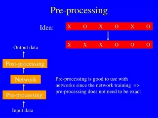
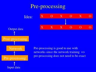
Pre-processing. X O X O X O. X X X O O O. Output data. Post-processing. Idea:. Network. Pre-processing is good to use with networks since the network training => pre-processing does not need to be exact. Pre-processing. Input data. Why Pre-process?

Pre-processing
E N D
Presentation Transcript
Pre-processing X O X O X O X X X O O O Output data Post-processing Idea: Network Pre-processing is good to use with networks since the network training => pre-processing does not need to be exact Pre-processing Input data
Why Pre-process? • Although in principlenetworks can approximate any function in practice its easier if pre-processing is performed first • Types of pre-processing: • 1. Linear transformations • e.g input normalisation • 2. Dimensionality reduction loss of info. Good pre-proc => lose irrelevant info and retain salient features • 3. Incorporate prior knowledge • look for edges / translational invariants
4. Feature extraction use a combination of input variables: can incorporate 1, 2 and 3 5. Feature selection decide which features to use
b e.g. Character recognition For a 256 x 256 character we have 65, 536 pixels. One input for each pixel is bad for many reasons: • Poor generalisation: data set would have to be vast to be able to properly constrain all the parameters (Curse of Dimensionality) • Takes forever to train • Answer: use e.g. averages of N2 pixels dimensionality reduction – each average could be a feature. • Which ones to use (select)? Use prior knowledge of where salient bits are for different letters
Be careful not to over-specify e.g if X was in one of k classes could use the posterior probabilities P(Ck| X) as features. Therefore, in principle only k-1 features are needed. In practice, its hard to obtain P(Ck| X) and so we would use a much larger number of features to ensure we don’t throw out the wrong thing Notice that the distinction between network training and pre-proc. is artificial: If we got all the posterior probs. the classification is complete. Leave some work for the network to do.
Input normalisation Useful for RBFNs (and MLPs): if variation in one parameter is small with respect to the others it will contribute very little to distance measures(l + e)2 ~ l2. Therefore, preprocess data to give zero mean and unit variance via simple transformation: x* = (x - m) s
However, this does not take into account correlations in the data. Can be better to use whitening (Bishop, 1995, pp 299-300)
Eigenvectors and eigenvalues If : Ax = lx For some scalar l not = to 0, then we say that x is an eigenvector with eigenvalue l. Clearly, x is not unique [e.g. if Ax = lx, A2x = l2x], so it is usual to scale x so that it has unit length. Intuition: direction of x is unchanged by being transformed by A so it in some sense reflects the principal axis of the transformation.
Eigenvector Facts If the data is D-dimensional there will be D eigenvectors If A is symmetric (true if A is the covariance matrix), the eigenvectors will be orthogonal and unit length so: xiT xj = 1 if i = j xiT xj = 0 else This means that the eigenvectors form a set of basis vectors. That is, any vector can be expressed as a linear sum of the eigenvectors.
LetU be a matrix whose columns are the eigenvectors uiof A, and La matrix with the corresponding eigenvalues li on the diagonals i.e: U = (u1, … …, un) And:L =diag(l1, ……, ln) So: AU = UL Because of orthogonality of the eigenvectorsU is orthonormal I.e: UT U = U-1 U = I (that is diag(1, ……, 1)) Thus we have the orthogonal similarity transformation: UT AU = UT U L = L By which we can transform A into a diagonal matrix
l1u1 l2u2 Also if A is the covariance matrix of multivariate normal data, eigenvectors/eigenvalues reflect the direction and extent of variation ie Standard deviation in each direction = eigenvalue
If A is diagonal, eigenvectors are oriented along the axes If A is the identity, A is circular
l1u1 l2u2 Whitening x* = L-1/2 UT (x - m) whereU is a matrix whose columns are the eigenvectors uiof S, the covariance matrix of the data, and L a matrix with the corresponding eigenvalues li on the diagonals and m is the mean of the data Why? Because the new covariance matrix will be approximately the identity matrix
Dimensionality Reduction • Clearly losing some information but this can be helpful due to curse of dimensionality • Need some way of deciding what dimensions to keep • Random choice • Principal components analysis (PCA) • Independent components analysis (ICA) • Self-organised maps (SOM) • etc
Random subset selection • Any suitable algorithm can be used especially ones used in selecting number of hidden units • Sequential forward search • Sequential backward search • Plus-l take away r • etc
Principle Components Analysis Transform the data into a lower dimensional space but lose as little information as possible Project the data onto unit vectors to reduce the dimensionality of the data. What vectors to use? x y || y || = 1 x* = xTy = yTx
l1u1 l2u2 Want to reduce the dimensionality of x from d to M x x x x x x x x
Therefore to minimise E we discard the dimensions with the smallest eigenvectors
PCA can also be motivated from considerations of the variance along an axis specified by the eigenvectors
PCA procedure: • Given a data set X = {x1, … … , xN} normalise the data (minus mean and divide by the std deviation) and calculate the covariance matrix C • Calculate the eigenvalues li and eigenvectors ui of C and order them from 1 to d in decending order starting with the largest eigenvalue • Discard the last d-M dimensions and transform the data via: Ie zi are the principal components (NB some books refer to the ui as the principal components)
Why use input normalisation? Must subtract the mean vector as the theory requires that the data are centred at the origin Also, we divide by the standard deviation as we must do something to ensure that input dimensions with a large range do not dominate the variance terms Why not use whitening? Since this removes the correlations that we are trying to find and makes all the eigenvalues similar
Should result in losing unnecessary information Here the data is best viewed along the dimension of the eigenvector with the most variance as this shows the 2 clusters clearly
But it is not guaranteed to work … Here projecting the data onto u1, the eigenvector with the most variance, loses all discriminatory information
Finally: How to decide M ie how many/which dimensions to leave out? This may be decided in advance due to constraints on processing power Another technique (used in eg Matlab) is to look at the contribution to the overall variance of each principal component and leave out any dimensions which fall below a certain threshold As ever, no one answer: may just want to try a few combinations or could even keep them all
PCA is very powerful in practical applications. But how do we compute eigenvectors and thus principal components in real situations? • Basically two ways: Batch and sequential • We have seen the batch method, but this can be impractical if the dimensionality or no. of data points is too large • Also in a nonstationary environment, sequential can track gradual changes in the data • It requires less storage space • Sequential mode is used in modelling self-organization • It mimics Hebbian learning rule …
Hebbian Learning Hebb's postulate of learning (or simply Hebb's rule) (1949), is the following: "When an axon of cell A is near enough to excite cell B and repeatedly or persistently takes part in firing it, some growth processes or metabolic changes take place in one or both cells such that A's efficiency as one of the cells firing B, is increased". then Ie if However, simple hebbian learning cause uncontrolled growth of weights to a max value so need to impose a normalisation constraint Where a is a +ve constant: known as Oja’s rule (1982) which makes |w|2 gradually relax to 1/ a – form of competition between synapses
In this way networks can exhibit selective amplification if there is one dominant eigenvector (cf PCA) How can such precise tuning come about? Hebbian learning
Relationship between PCA and Hebbian learning Consider a single neuron with a Hebbian learning rule: w1(t) input x(t) output y(t) = wT(t) x(t) wd(t) Oja’s learning rule (Oja, 1982) : wi(t+1) = wi(t)+ hy(t) (xi(t)–y 2(t) wi (t)) Where y(t) xi (t)is the Hebbian termand – y2(t) wi (t)is the normalisation termwhich avoids uncontrolled growth of the weights (=> ||w|| = 1 at convergence)
This can be shown to have a stable minimum at • Cw = l 1 w • Where C is the the covariance matrix of the training data . Result: w(t) converges to wthe eigenvector of C which has the largest eigenvalue l 1 . • The output is therefore : • y = wTx = u1Tx • Ie the first principal component of C • Thus a single linear neuron with a Hebbian learning rule can evolve into a filter for the first principal component • Intuitively, consider the 1D case: here the eigenvectorw is either 1 or –1. At convergence of Oja’s learning rule we have: • y(t) (x-y(t) w(t))=0which is satisfied ifw(t)=1 or -1
We now introduce a special PCA learning rule called APEXdeveloped by Kung and Diamantaras, 1990. This is a generalisation of the single neuron case to multiple neurons where the outputs are connected via inhibitory links w11(t) y1(t) w1d(t) aj1(t) input x(t) y2(t) ajd(t) wdd(t) output j: yj(t) = wjT(t) x(t) + ajT(t) yj-1(t) Where we define the feedback vector: yj-1= [y1(t), y2(t) , … yj-1(t)] Wj(t) = [wj1(t), wj2(t) , … wjd(t)] and aj(t) = [aj1(t), aj2(t) , … ajd(t)]
Where the update rules for wj and ajare: wj(t+1) = wj(t) + h yj(t) (x(t) -y2j(t) wj(t)) (Hebbian + normalisation) aj(t+1) = aj(t)- h yj(t)(yj-1(t)+y2j(t) aj(t)) (anti-Hebbian (inhibitory) + normalisation) Procedure to find the yi (ie the principal components) is analogous to proof by induction: if we have found (y1 , y1 , … yi-1 ) we can determine the feedback vector: yi-1(t)=[y1(t), ...., yj-1(t)]
Apex algorithm 1. Initialize the feedforward weight vector wj and the feedback weight vector aj to small random values at time t = 1, where j = 1, 2, …, d. Assign a small positive value for h. 2. Set j=1 and compute the first principal component y1 as for the single neuron ie for t = 1, 2, 3, … compute: y1(t) = w1T(t) x(t) w1(t+1) = w1(t)+ h y1(t) (x(t)-y1(t) w1(t)) (Continued overleaf …)
Set j=2 and for t = 1, 2, 3, … compute: • yj-1(t)=[y1(t), ...., yj-1(t)] (the feedback) • yj(t) = wjT(t) x(t) + ajT(t) yj-1(t) • wj(t+1) = wj(t) + h yj(t) (x(t) -yj(t) wj(t)) • aj(t+1) = aj(t)- h yj(t)(yj-1(t)+yj(t) aj(t)) • 4. Increase j by 1 and go to step 3. Repeat till j = M the desired number of dimensions
Theoretically, PCA is the optimal (in terms of not losing information) way to encode high dimensional data onto a lower dimensional subspace Can be used for data compression where intuition is that getting rid of dimensions with little variance gets rid of noise
Independent Components Analysis (ICA) As the name implies, an extension of PCA but rooted in information theory. Starting point: suppose we have the following situation: Observation vector x(n) Demixer W Mixer A Output vector y(n) Source vector u(n) Unknown environment
That is we have a number of vectors of values (indexed by n eg data at various time-steps) generated by d independent sources u(n) = (u1 (n), …, ud (n) ) (assumed to have zero mean) which have been mixed by a d x d matrix A to give a vector of observations: x(n) = (x1 (n), …, xd (n) ) (also zero mean as u zero mean). That is: x (n) = A u (n) Where A and u(n) are unknown. The problem is to recover u when all we know (all we can see) are the observation vectors x Problem therefore known as blind source separation
Example: u1 (t) = 0.1 sin (400 t )cos( 30 t) u2 (t) = 0.001 sign (sin(500 t+ 9cos (40 t))) u3 (t) = uniformally distributed noise in the range [-1,1] x1 (t) = 0.56 u1 (t) + 0.79 u2 (t) -0.37 u3 (t) x2 (t) = -0.75 u1 (t) + 0.65 u2 (t) +0.86 u3 (t) x3 (t) = 0.17 u1 (t) + 0.32 u2 (t) -0.48 u3 (t) Problem: we receive signals x(t), how do we recover u(t)?
u1(t) u2(t) u3(t)
x1(t) x2(t) x3(t)
To solve this we need to find a matrix Wsuch that: y(n) =W x(n) with the property thatu can be recovered from the outputs y. Thus the blind source separation problem can be stated as: Given N independent realisations of the observation vector x, find an estimate for the inverse of the mixing matrix A since : y(n) =W x(n) = A-1x(n) = A-1A u(n) =u(n)
Neurobiological correlate:the cocktail party problem The brain has the ability to to selectively tune to and follow one of a number of (independent) voices despite noise, delays, water in your ear lecturer droning on etc etc Very many applications including: Speech analysis for eg teleconferencing Financial analysis: extract the underlying set of dominant components Medical sensor interpretation: eg separate a foetuses heartbeat from the mothers (Sussex) neuroscience (Ossorio, Baddeley and Anderson): analysis of cuttlefish patterns. Try to find an underlying alphabet/language of patterns used to convey information
Use Independent Component Analysis (Comon, 1994) Can be viewed as an extension of PCA as both aim to find linear sums of components to re-represent the data In ICA, however, we impose statistical independence on the vectors found and lose the orthogonality constraint Definition: random variables X and Y are statistically independent if joint probability density function can be expressed as a product of the marginal density functions (ie pdf’s of X and Y as if they were on their own): f(x, y) = f(x) f(y) [NB discrete analogy: if A and B are independent events then: P(A and B) = P(A, B) = P(A) P(B) ]
PCA ICA PCA good for gaussian data, ICA good for non gaussian as indpendence => non-gaussianity In fact, independent components MUST be nongaussian (more interesting distributions if non-gaussian) and to get components we maximise the non-gaussianity (the kurtosis) of the data Why? Because a linear sum of gaussians is itself gaussian and one cannot distinguish the components from the mixture model
Young field (mid 90’s), still developing, somewhat in concurrence with kernel techniques (eg kernel PCA and kernel ICA: find non-linear combinations of components to represent the data) Need some measure of statistical independence of X and Y: Can use mutual information I(X, Y) Concept from information theory: defined in terms of entropy which is a measure of the average amount of information a variable conveys, or analogously our uncertainty about the variable If X is the system input and Y the system output, the mutual information I(X, Y) is the difference in our levels of uncertainty about the system input (it’s entropy) before and after observing the system output. Thus if : I(X, Y) = 0 X and Y are statistically independent [or intuitively: no information about X from Y and vice versa => X, Y independent]
Idea, therefore is to minimise the mutual info I(yi,, yj) between all pairs I and j of the outputs (which we want to be equal to the original inputs which are independent) This is equivalent to minimising the Kullback-Leibler (KL) divergence which measures the difference between the joint pdf f(y,W) and the product of the marginal densities f(yi,W) with respect to W. Thus we have (a variant of) the Infomax Principle (Comon): Given a d-by-1 vector x representing a linear combination of d independent source signals, the transformation of the observation vector x by a neural system into a new vector y should be carried out in a way that the KL divergence between the paramaterised probability density function f(y,W) and the product of the marginal densities f(yi,W) is minimised with respect to the unknown parameter matrix W
Which after some hard maths (Haykin 10.11 and other bits of chapter 10) leads us to the following algorithm for finding W • W(n +1)- W(n)= h( n) [I- f(y(n))yT(n)] W(n) • where: • (y) = [f (y1), f (y2) , …, f (ym)]T And: NB h must be chosen to be sufficiently small for stability of the algorithm (see Haykin). Many other versions are available (FastICA seems quite good) Return to the problem described earlier …
u1 (t) = 0.1 sin (400 t )cos( 30 t) u2 (t) = 0.001 sign (sin(500 t+ 9cos (40 t))) u3 (t) = uniformally distributed noise in the range [-1,1] x1 (t) = 0.56 u1 (t) + 0.79 u2 (t) -0.37 u3 (t) x2 (t) = -0.75 u1 (t) + 0.65 u2 (t) +0.86 u3 (t) x3 (t) = 0.17 u1 (t) + 0.32 u2 (t) -0.48 u3 (t) Problem: we receive signals x(t), how do we recover u(t)?
u1(t) u2(t) u3(t)
x1(t) x2(t) x3(t)
Using the blind separation learning rule starting from random weights in the range [0, 0.05], h =0.1, N=65000, timestep = 1x 10⁻⁴, batch version of algorithm for stability (Haykin, p.544): 0.0109 0.0340 0.0260 W(0)= 0.0024 0.0467 0.0415 0.0339 0.0192 0.0017 0.2222 0.0294 -0.6213 W(t) converges to -10.1932 -9.8131 -9.7259 around t=300 4.1191 -1.7879 -6.3765 2.5 0 0 where WA ~ 0 17.5 0 0 0 0.24 W is almost an inverse of A (with scaling of the original signals as the solution not unique) and so the signal is recovered