Download
1 / 53
540 likes | 716 Vues
Atmospheric muons & neutrinos in neutrino telescopes. Neutrino oscillations Muon & neutrino beams Muons & neutrinos underground. p. p. m. e. n e. n m. n m. Atmospheric neutrinos. Produced by cosmic-ray interactions Last component of secondary cosmic radiation to be measured

E N D
Atmospheric muons & neutrinos in neutrino telescopes Neutrino oscillations Muon & neutrino beams Muons & neutrinos underground Tom Gaisser Cosmic rays - 2
p p m e ne nm nm Atmospheric neutrinos • Produced by cosmic-ray interactions • Last component of secondary cosmic radiation to be measured • Close genetic relation with muons • p + A p± (K±) + other hadrons • p± (K±) m± + nm (nm) • m± e± + nm (nm) + ne (ne) Tom Gaisser Cosmic rays - 2
Historical context • Detection of atmospheric neutrinos • Markov (1960) suggests Cherenkov light in deep lake or ocean to • detect atmospheric n interactions for neutrino physics • Greisen (1960) suggests water Cherenkov detector in deep mine • as a neutrino telescope for extraterrestrial neutrinos • First recorded events in deep mines with electronic detectors, 1965: • CWI detector (Reines et al.); KGF detector (Menon, Miyake et al.) • Two methods for calculating atmospheric neutrinos: • From muons to parent pions infer neutrinos (Markov & Zheleznykh, 1961; Perkins) • From primaries to p, K and m to neutrinos (Cowsik, 1965 and most later calculations) • Essential features known since 1961: Markov & Zheleznykh, Zatsepin & Kuz’min • Monte Carlo calculations follow second method • Stability of matter: search for proton decay, 1980’s • IMB & Kamioka -- water Cherenkov detectors • KGF, NUSEX, Frejus, Soudan-- iron tracking calorimeters • Principal background is interactions of atmospheric neutrinos • Need to calculate flux of atmospheric neutrinos Tom Gaisser Cosmic rays - 2
Historical context (cont’d) • Atmospheric neutrino anomaly - 1986, 1988 … • IMB too few m decays (from interactions of nm) 1986 • Kamioka m-like / e-like ratio too small. • Neutrino oscillations first explicitly suggested in 1988 Kamioka paper • IMB stopping / through-going consistent with no oscillations (1992) • Hint of pathlength dependence from Kamioka, Fukuda et al., 1994 • Discovery of atmospheric neutrino oscillations by S-K • Super-K: “Evidence for neutrino oscillations” at Neutriino 98 • Subsequent increasingly detailed analyses from Super-K: nm nt • Confirming evidence from MACRO, Soudan, K2K, MINOS • Analyses based on ratios comparing to 1D calculations • Compare up vs down • Parallel discovery of oscillations of Solar neutrinos • Homestake 1968-1995, SAGE, Gallex … chemistry counting expts. • Kamioka, Super-K, SNO … higher energy with directionality • ne ( nm, nt ) Tom Gaisser Cosmic rays - 2
p p m e nm ne nm ( ) 1.27 L(km) dm2(eV2) En(GeV) P(nmnt) = sin22q sin2 Atmospheric neutrino beam • Cosmic-ray protons produce neutrinos in atmosphere • nm/ne ~ 2 for En < GeV • Up-down symmetric • Oscillation theory: • Characteristic length (E/dm2) • related to dm2 =m12 – m22 • Mixing strength (sin22q) • Compare 2 pathlengths • Upward: 10,000 km • Downward: 10 – 20 km Wolfenstein; Mikheyev & Smirnov Tom Gaisser Cosmic rays - 2
e (or m) ne (or nm) nm Classes of atmospheric n events m Contained (any direction) n-induced m (from below) External events Plot is for Super-K but the classification is generic Contained events Tom Gaisser Cosmic rays - 2
Super-K atmospheric neutrino data (hep-ex/0501064) CC ne CC nm 1489day FC+PC data + 1646day upward going muon data Tom Gaisser Cosmic rays - 2
0 0 • 0 C23 S23 • 0 -S23 C23 C13 0 S13 0 1 0 -S13 0 C13 C12 S12 0 -S12 C12 0 0 0 1 U = “atmospheric” “solar” C13 ~ 1 S13 small Atmospheric n nm nt, dm2 = 2.5 x 10⁻³ eV2 maximal mixing Solar neutrinos ne{nm,nt}, dm2 ~ 10-4 eV2 large mixing Yumiko Takenaga, ICRC2007 3-flavor mixing Flavor state | na ) = Si Uai | ni ), where | ni ) is a mass eigenstate Tom Gaisser Cosmic rays - 2
High-energy Neutrino telescopes Large volume--coarse instrumentation--high energy (> TeV) as compared to Super-K with 40% photo-cathode over 0.05 Mton Tom Gaisser Cosmic rays - 2
Detecting neutrinos in H20Proposed by Greisen, Markov in 1960 • Heritage: • DUMAND • IMB • Kamiokande Super-K ANTARES SNO IceCube Tom Gaisser Cosmic rays - 2
Expected flux of relic supernova neutrinos Lines show atmospheric neutrinos + antineutrinos Astrophysical neutrinos (WB “bound” / 2 for osc) nm ne Solar n RPQM for prompt n from charm Bugaev et al., PRD58 (1998) 054001 Slope = 2.7 Prompt n Cosmogenic neutrinos Slope = 3.7 The neutrino landscape Tom Gaisser Cosmic rays - 2
The atmosphere The atmosphere (exponential approximation) Pressure = Xv = Xo exp{ -hv / ho } , where ho = 6.4 km for Xv < 200 g / cm2 and X0 = 1030 g / cm2 Density = r = -dXv / dhv = Xv / ho Xv ~ p = rRT ho ~ RT Tom Gaisser Cosmic rays - 2
Cascade equations For hadronic cascades in the atmosphere X = depth into atmosphere d = decay length l = Interaction length • Fji( Ei,Ej) has no explicit dimension, so F F(x) • x = Ei/Ej & ∫…F(Ei,Ej) dEj / Ei ∫…F(x) dx / x2 • Small scaling violations from mi, LQCD ~ GeV, etc • Still… a remarkably useful approximation Tom Gaisser Cosmic rays - 2
EAS Boundary condition for inclusive flux Boundary conditions Tom Gaisser Cosmic rays - 2
Example: flux of nucleons Approximate: l ~ constant, leading nucleon only Separate X- and E-dependence; try factorized solution, N(E,X) = f (E) · g(X), f (E) ~ E –(g+1) Separation constant LN describes attenuation of nucleons in atmosphere Uncorrelated fluxes in atmosphere Tom Gaisser Cosmic rays - 2
Evaluate LN: Flux of nucleons: K fixed by primary spectrum at X = 0 Nucleon fluxes in atmosphere N(E, X) = N(E, 0) x exp{-X/LN} Tom Gaisser Cosmic rays - 2
Account for p n CAPRICE98 (E. Mocchiutti, thesis) Comparison to proton fluxes Tom Gaisser Cosmic rays - 2
pion decay probability p± in the atmosphere p decay or interaction more probable for E < ep or E > ep = 115 GeV Tom Gaisser Cosmic rays - 2
p± (K±) in the atmosphere • Low-energy limit: Ep < ep ~ 115 GeV Tom Gaisser Cosmic rays - 2
p± (K±) in the atmosphere • High-energy limit: Ep > ep ~ 115 GeV Spectrum of decaying pions one power steeper for Ep >> ep Tom Gaisser Cosmic rays - 2
m and nm in the atmosphere • To calculate spectra of m and n • Multiply P(E,X) by pion decay probability • Include contribution of kaons • Dominant source of neutrinos • Integrate over kinematics of p m + nm and K m + nm • Integrate over the atmosphere (X) • Good description of data Tom Gaisser Cosmic rays - 2
2-body decays of p± and K± • p+ m+ + nm 99.99% • K+ m+ + nm 63.44% • also for negative mesons • to produce anti-neutrinos In rest frame of parent m and n have equal and opposite 3 momentum p CM energy of neutrino = p = |p| = En* = (M2 – m2) / (2 M) CM energy of muon = p2 + m2 = Em* = (M2 + m2) / (2 M) M = mass of parent meson, m = mass of muon For both m and n : ELAB = g E* + b g p cos(q) Tom Gaisser Cosmic rays - 2
Momentum distributions for p, K ELAB = g E* + b g p cos(q*) g = EM / M and assume ELAB >> M so b 1 Then (E* - p) / M < ELAB / EM < (E* + p) / M because -1 < cos(q*) < 1 Also, decay is isotropic in rest frame so dn / d cos(q*) = constant But d ELAB = d cos(q*) , so dn / d ELAB = constant Normalization requires exactly one m or n so the normalization gives (constant)-1 = EM ( 1 – r ) where r = m2 / M2 for both m and n Note: rp = 0.572 while rK = 0.0458, an important difference ! Tom Gaisser Cosmic rays - 2
Compare m and n Tom Gaisser Cosmic rays - 2
m and nm differ only by kinematics of p± and K± decay Tom Gaisser Cosmic rays - 2
(g-1) Zab≡∫x Fab(x) dx Spectrum-weighted moments Tom Gaisser Cosmic rays - 2
Relative magnitude of li and di = X cosq ( E / ei ) determines competition between interaction and decay Xv = 100 g / cm2 at 15 km altitude which is comparable to interaction lengths of hadrons in air Interaction vs. decay Tom Gaisser Cosmic rays - 2
Kaons produce most nm for 100 GeV < En < 100 TeV High-energy atmospheric neutrinos Primary cosmic-ray spectrum (nucleons) Nucleons produce pions kaons charmed hadrons that decay to neutrinos Eventually “prompt n” from charm decay dominate, ….but what energy? Tom Gaisser Cosmic rays - 2
vertical 60 degrees Importance of kaons at high E • Importance of kaons • main source of n > 100 GeV • p K+ + L important • Charmed analog important for prompt leptons at higher energy Tom Gaisser Cosmic rays - 2
Neutrinos from kaons Critical energies determine where spectrum changes, but AKn / Apn and ACn / AKn determine magnitudes New information from MINOS relevant to nm with E > TeV Tom Gaisser Cosmic rays - 2
Electron neutrinos K+ p0ne e± ( B.R. 5% ) KL0 p±ne e( B.R. 41% ) Kaons important for ne down to ~10 GeV Tom Gaisser Cosmic rays - 2
x 1.37 x 1.27 TeV m+/m- with MINOS far detector • 100 to 400 GeV at depth > TeV at production • Increase in charge ratio shows • p K+L is important • Forward process • s-quark recombines with leading di-quark • Similar process for Lc? Increased contribution from kaons at high energy Tom Gaisser Cosmic rays - 2
Z-factors assumed constant for E > 10 GeV • Energy dependence of charge ratio comes from • increasing contribution of kaons in TeV range • coupled with fact that charge asymmetry is larger for • kaon production than for pion production • Same effect larger for nm / nm because kaons dominate MINOS fit ratios of Z-factors Tom Gaisser Cosmic rays - 2
Atmospheric neutrinos – harder spectrum from kaons? AMANDA atmospheric neutrino arXiv:0902.0675v1 Re-analysis of Super-K Gonzalez-Garcia, Maltoni, Rojo JHEP 2007 Tom Gaisser Cosmic rays - 2
Signature of charm: q dependence For eK < E cos(q) < ec , conventional neutrinos ~ sec(q) , but “prompt” neutrinos independent of angle Uncertain charm component most important near the vertical Tom Gaisser Cosmic rays - 2
Gelmini, Gondolo, Varieschi PRD 67, 017301 (2003) Neutrinos from charm • Main source of atmospheric n for En > ?? • ?? > 20 TeV • Large uncertainty in normalization! • References: Higher charm production: Bugaev, E. V., A. Misaki, V. A. Naumov, T. S. Sinegovskaya, S. I. Sinegovsky, and N. Takahashi, Phys. Rev. D, 58, 054001 (1998) . Lower level of charm production R. Enberg, M.H. Reno & I. Sarcevic, PRD 78, 043005 (2008). Tom Gaisser Cosmic rays - 2
Charm in astrophysical sources See Elisa Resconi’s lecture, Refs to Kelner & Aharonian • Depends on environment • Target photon density for p g N p • Gas density for p p p, p, K, … • The same target densities determine the competition between decay and interaction for p n, K n & D n Enberg, R., M. H. Reno, and I. Sarcevic, Phys. Rev. D, 79, 053006, 2009. Tom Gaisser Cosmic rays - 2
Muons & Neutrinos underground Muon average energy loss: from Reviews of Particle Physics, Cosmic Rays Critical energy: Tom Gaisser Cosmic rays - 2
Shallow: Deep: m energy spectrum underground Average relation between energy at surface and energy underground Tom Gaisser Cosmic rays - 2
High-energy, deep muons Tom Gaisser Cosmic rays - 2
Differential and integral spectrum of atmospheric muons Differential Integral Energy loss: Em (surface) = exp{ b X } · ( Em +e ) - e Set Em = e { exp[ b X ] - 1 } in Integral flux to get depth – intensity curve Tom Gaisser Cosmic rays - 2
Plot shows dNm / dln(Em) Tom Gaisser Cosmic rays - 2
Detecting neutrinos • Rate = Neutrino flux x Absorption in Earth x Neutrino cross section x Size of detector x Range of muon (for nm) • (Range favors nm channel) Probability to detect nm-induced m Tom Gaisser Cosmic rays - 2
Neutrino effective area • Rate: = ∫fn(En)Aeff(En)dEn • Earth absorption • Starts 10-100 TeV • Biggest effect near vertical • Higher energy n’s absorbed at larger angles Tom Gaisser Cosmic rays - 2
Neutrino-induced muons Tom Gaisser Cosmic rays - 2
Atmospheric muons (shape only) Atmospheric Tom Gaisser Cosmic rays - 2
Million to 1 background to signal from above. Use Earth as filter; look for neurtinos from below. Muons in n telescopes Downward atmospheric muons Neutrino-induced muons from all directions SNO at 6000 m.w.e. depth Tom Gaisser Cosmic rays - 2
Muons in IceCube Downward atmospheric muons Neutrino-induced muons from all directions IceCube P. Berghaus et al., ISVHECRI-08 also HE1.5 ~75° for deepest Mediterranean site Crossover at ~85° for shallow detectors Tom Gaisser Cosmic rays - 2 48
preliminary Atmospheric m and n in IceCubeExtended energy reach of km3 detector Dmitry Chirkin, ICRC 2009 Currently limited by systematics Patrick Berkhaus, ICRC 2009 Tom Gaisser Cosmic rays - 2
pion decay probability Deep muons as a probe of weather in the stratosphere • Barrett et al. • MACRO • MINOS far detector • Sudden stratospheric warmings observed • IceCube • Interesting because of unique seasonal features of the upper atmosphere over Antarctica related to ozone hole • Decay probability ~ T: • h0 ~ RT Tom Gaisser Cosmic rays - 2