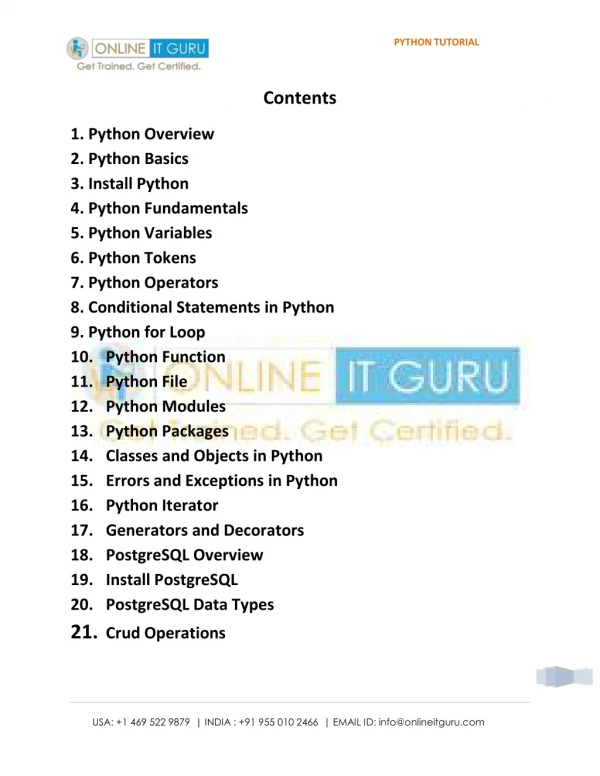
A Brief Python Tutorial
A Brief Python Tutorial. Sven H. Chilton University of California - Berkeley LBL Heavy Ion Fusion Group Talk 16 August, 2007. Outline. Why Use Python? Running Python Types and Operators Basic Statements Functions Scope Rules (Locality and Context) Some Useful Packages and Resources.

A Brief Python Tutorial
E N D
Presentation Transcript
A Brief Python Tutorial Sven H. Chilton University of California - Berkeley LBL Heavy Ion Fusion Group Talk 16 August, 2007
Outline Why Use Python? Running Python Types and Operators Basic Statements Functions Scope Rules (Locality and Context) Some Useful Packages and Resources
Python is object-oriented Structure supports such concepts as polymorphism, operation overloading, and multiple inheritance It's free (open source) Downloading and installing Python is free and easy Source code is easily accessible Free doesn't mean unsupported! Online Python community is huge It's portable Python runs virtually every major platform used today As long as you have a compatible Python interpreter installed, Python programs will run in exactly the same manner, irrespective of platform It's powerful Dynamic typing Built-in types and tools Library utilities Third party utilities (e.g. Numeric, NumPy, SciPy) Automatic memory management Why Use Python? (1)
Why Use Python? (2) • It's mixable • Python can be linked to components written in other languages easily • Linking to fast, compiled code is useful to computationally intensive problems • Python is good for code steering and for merging multiple programs in otherwise conflicting languages • Python/C integration is quite common • WARP is implemented in a mixture of Python and Fortran • It's easy to use • Rapid turnaround: no intermediate compile and link steps as in C or C++ • Python programs are compiled automatically to an intermediate form called bytecode, which the interpreter then reads • This gives Python the development speed of an interpreter without the performance loss inherent in purely interpreted languages • It's easy to learn • Structure and syntax are pretty intuitive and easy to grasp
In addition to being a programming language, Python is also an interpreter. The interpreter reads other Python programs and commands, and executes them. Note that Python programs are compiled automatically before being scanned into the interpreter. The fact that this process is hidden makes Python faster than a pure interpreter. How to call up a Python interpreter will vary a bit depending on your platform, but in a system with a terminal interface, all you need to do is type “python” (without the quotation marks) into your command line. Example: # From here on, the $ sign denotes the start of a terminal command line, and the # sign denotes a comment. Note: the # sign denotes a comment in Python. Python ignores anything written to the right of a # sign on a given line $ python# Type python into your terminal's command line >>># After a short message, the >>> symbol will appear. This signals # the start of a Python interpreter's command line Running Python (1)
Running Python (2) Once you're inside the Python interpreter, type in commands at will. Examples: >>> print 'Hello world' Hello world # Relevant output is displayed on subsequent lines without the >>> symbol >>> x = [0,1,2] # Quantities stored in memory are not displayed by default >>> x # If a quantity is stored in memory, typing its name will display it [0,1,2] >>> 2+3 5 >>> # Type ctrl-D to exit the interpreter $
Running Python (3) Python scripts can be written in text files with the suffix .py. The scripts can be read into the interpreter in several ways: Examples: $ python script.py # This will simply execute the script and return to the terminal afterwards $ python -i script.py # The -i flag keeps the interpreter open after the script is finished running $ python >>> execfile('script.py') # The execfile command reads in scripts and executes them immediately, as though they had been typed into the interpreter directly $ python >>> import script # DO NOT add the .py suffix. Script is a module here # The import command runs the script, displays any unstored outputs, and creates a lower level (or context) within the program. More on contexts later.
Running Python (4) Suppose the file script.py contains the following lines: print 'Hello world' x = [0,1,2] Let's run this script in each of the ways described on the last slide: Examples: $ python script.py Hello world $ # The script is executed and the interpreter is immediately closed. x is lost. $ python -i script.py Hello world >>> x [0,1,2] >>> # “Hello world” is printed, x is stored and can be called later, and the interpreter is left open
Examples: (continued from previous slide) $ python >>> execfile('script.py') Hello world >>> x [0,1,2] >>> # For our current purposes, this is identical to calling the script from the terminal with the command python -i script.py $ python >>> import script Hello world >>> x Traceback (most recent call last): File "<stdin>", line 1, in ? NameError: name 'x' is not defined >>> # When script.py is loaded in this way, x is not defined on the top level Running Python (5)
Running Python (6) Examples: (continued from previous slide) # to make use of x, we need to let Python know which module it came from, i.e. give Python its context >>> script.x [0,1,2] >>> # Pretend that script.py contains multiple stored quantities. To promote x (and only x) to the top level context, type the following: $ python >>> from script import x Hello world >>> x [0,1,2] >>> # To promote all quantities in script.py to the top level context, type from script import * into the interpreter. Of course, if that's what you want, you might as well type python -i script.py into the terminal.
Types and Operators: Types of Numbers (1) Python supports several different numeric types Integers Examples: 0, 1, 1234, -56 Integers are implemented as C longs Note: dividing an integer by another integer will return only the integer part of the quotient, e.g. typing 7/2 will yield 3 Long integers Example: 999999999999999999999L Must end in either l or L Can be arbitrarily long Floating point numbers Examples: 0., 1.0, 1e10, 3.14e-2, 6.99E4 Implemented as C doubles Division works normally for floating point numbers: 7./2. = 3.5 Operations involving both floats and integers will yield floats: 6.4 – 2 = 4.4
Types and Operators: Types of Numbers (2) Other numeric types: Octal constants Examples: 0177, -01234 Must start with a leading 0 Hex constants Examples: 0x9ff, 0X7AE Must start with a leading 0x or 0X Complex numbers Examples: 3+4j, 3.0+4.0j, 2J Must end in j or J Typing in the imaginary part first will return the complex number in the order Re+ImJ
Basic algebraic operations Four arithmetic operations: a+b, a-b, a*b, a/b Exponentiation: a**b Other elementary functions are not part of standard Python, but included in packages like NumPy and SciPy Comparison operators Greater than, less than, etc.: a < b, a > b, a <= b, a >= b Identity tests: a == b, a != b Bitwise operators Bitwise or: a | b Bitwise exclusive or: a ^ b # Don't confuse this with exponentiation Bitwise and: a & b Shift a left or right by b bits: a << b, a >> b Other Not surprisingly, Python follows the basic PEMDAS order of operations Python supports mixed-type math. The final answer will be of the most complicated type used. Types and Operators: Operations on Numbers
Types and Operators: Strings and Operations Thereon Strings are ordered blocks of text Strings are enclosed in single or double quotation marks Double quotation marks allow the user to extend strings over multiple lines without backslashes, which usually signal the continuation of an expression Examples: 'abc', “ABC” Concatenation and repetition Strings are concatenated with the + sign:>>> 'abc'+'def''abcdef' Strings are repeated with the * sign:>>> 'abc'*3'abcabcabc'
Types and Operators: Indexing and Slicing (1) Indexing and slicing Python starts indexing at 0. A string s will have indexes running from 0 to len(s)-1 (where len(s) is the length of s) in integer quantities. s[i] fetches the ith element in s>>> s = 'string'>>> s[1] # note that Python considers 't' the first element 't' # of our string s s[i:j] fetches elements i (inclusive) through j (not inclusive)>>> s[1:4]'tri' s[:j] fetches all elements up to, but not including j>>> s[:3]'str' s[i:] fetches all elements from i onward (inclusive)>>> s[2:]'ring'
Types and Operators: Indexing and Slicing (2) Indexing and slicing, contd. s[i:j:k] extracts every kth element starting with index i (inlcusive) and ending with index j (not inclusive)>>> s[0:5:2]'srn' Python also supports negative indexes. For example, s[-1] means extract the first element of s from the end (same as s[len(s)-1])>>> s[-1]'g'>>> s[-2]'n' Python's indexing system is different from those of Fortan, MatLab, and Mathematica. The latter three programs start indexing at 1, and have inclusive slicing, i.e. the last index in a slice command is included in the slice
Types and Operators: Lists Basic properties: Lists are contained in square brackets [] Lists can contain numbers, strings, nested sublists, or nothing Examples: L1 = [0,1,2,3], L2 = ['zero', 'one'], L3 = [0,1,[2,3],'three',['four,one']], L4 = [] List indexing works just like string indexing Lists are mutable: individual elements can be reassigned in place. Moreover, they can grow and shrink in place Example: >>> L1 = [0,1,2,3]>>> L1[0] = 4>>> L1[0]4
Types and Operators: Operations on Lists (1) Some basic operations on lists: Indexing: L1[i], L2[i][j] Slicing: L3[i:j] Concatenation:>>> L1 = [0,1,2]; L2 = [3,4,5]>>> L1+L2[0,1,2,3,4,5] Repetition:>>> L1*3[0,1,2,0,1,2,0,1,2] Appending: >>> L1.append(3)[0,1,2,3] Sorting: >>> L3 = [2,1,4,3]>>> L3.sort()[1,2,3,4]
Types and Operators: Operations on Lists (2) More list operations: Reversal:>>> L4 = [4,3,2,1]>>> L4.reverse()>>> L4[1,2,3,4] Shrinking:>>> del L4[2]>>> Lx[i:j] = [] Index and slice assignment:>>> L1[1] = 1>>> L2[1:4] = [4,5,6] Making a list of integers: >>> range(4)[0,1,2,3]>>> range(1,5)[1,2,3,4]
Types and Operators: Tuples Basic properties: Tuples are contained in parentheses () Tuples can contain numbers, strings, nested sub-tuples, or nothing Examples: t1 = (0,1,2,3), t2 = ('zero', 'one'), t3 = (0,1,(2,3),'three',('four,one')), t4 = () As long as you're not nesting tuples, you can omit the parenthesesExample: t1 = 0,1,2,3 is the same as t1 = (0,1,2,3) Tuple indexing works just like string and list indexing Tuples are immutable: individual elements cannot be reassigned in place. Concatenation: >>> t1 = (0,1,2,3); t2 = (4,5,6)>>> t1+t2(0,1,2,3,4,5,6) Repetition:>>> t1*2(0,1,2,3,0,1,2,3) Length: len(t1) (this also works for lists and strings)
Types and Operators: Arrays (1) Note: arrays are not a built-in python type; they are included in third-party packages such as Numeric and NumPy. However, they are very useful to computational math and physics, so I will include a discussion of them here. Basic useage: Loading in array capabilities: # from here on, all operations involving arrays assume you have already made this step>>> from numpy import * Creating an array:>>> vec = array([1,2,3]) Creating a 3x3 matrix:>>> mat = array([[1,2,3],[4,5,6],[7,8,9]]) If you need to initialize a dummy array whose terms will be altered later, the zeros and ones commands are useful; zeros((m,n),'typecode') will create an m-by-n array of zeros, which can be integers, floats, double precision floats etc. depending on the type code used
Types and Operators: Arrays (2) Arrays and lists have many similarities, but there are also some important differences Similarities between arrays and lists: Both are mutable: both can have elements reassigned in place Arrays and lists are indexed and sliced identically The len command works just as well on arrays as anything else Arrays and lists both have sort and reverse attributes Differences between arrays and lists: With arrays, the + and * signs do not refer to concatenation or repetition Examples:>>> ar1 = array([2,4,6])>>> ar1+2 # Adding a constant to an array adds the constant to each term [4,6,8,] # in the array>>> ar1*2 # Multiplying an array by a constant multiplies each term in [4,8,12,] # the array by that constant
More differences between arrays and lists: Adding two arrays is just like adding two vectors>>> ar1 = array([2,4,6]); ar2 = array([1,2,3])>>> ar1+ar2 [3,6,9,] Multiplying two arrays multiplies them term by term:>>> ar1*ar2[2,8,18,] Same for division:>>> ar1/ar2[2,2,2,] Assuming the function can take vector arguments, a function acting on an array acts on each term in the array>>> ar2**2[1,4,9,]>>> ar3 = (pi/4)*arange(3) # like range, but an array>>> sin(ar3)[ 0. , 0.70710678, 1. ,] Types and Operators: Arrays (3)
More differences between arrays and lists: The biggest difference between arrays and lists is speed; it's much faster to carry out operations on arrays (and all the terms therein) than on each term in a given list.Example: take the following script:tt1 = time.clock()sarr = 1.*arange(0,10001)/10000; sinarr = sin(sarr)tt2 = time.clock()slist = []; sinlist = []for i in range(10001): slist.append(1.*i/10000) sinlist.append(sin(slist[i]))tt3 = time.clock()Running this script on my system shows that tt2-tt1 (i.e., the time it takes to set up the array and take the sin of each term therein) is 0.0 seconds, while tt3-tt2 (the time to set up the list and take the sin of each term therein) is 0.26 seconds. Types and Operators: Arrays (4)
Types and Operators: Mutable vs. Immutable Types (1) Mutable types (dictionaries, lists, arrays) can have individual items reassigned in place, while immutable types (numbers, strings, tuples) cannot. >>> L = [0,2,3] >>> L[0] = 1 >>> L [1,2,3] >>> s = 'string' >>> s[3] = 'o' Traceback (most recent call last): File "<stdin>", line 1, in ? TypeError: object does not support item assignment However, there is another important difference between mutable and immutable types; they handle name assignments differently. If you assign a name to an immutable item, then set a second name equal to the first, changing the value of the first name will not change that of the second. However, for mutable items, changing the value of the first name will change that of the second. An example to illustrate this difference follows on the next slide.
Immutable and mutable types handle name assignments differently >>> a = 2 >>> b = a # a and b are both numbers, and are thus immutable >>> a = 3 >>> b 2 Even though we set b equal to a, changing the value of a does not change the value of b. However, for mutable types, this property does not hold. >>> La = [0,1,2] >>> Lb = La # La and Lb are both lists, and are thus mutable >>> La = [1,2,3] >>> Lb [1,2,3] Setting Lb equal to La means that changing the value of La changes that of Lb. To circumvent this property, we would make use of the function copy.copy(). >>> La = [0,1,2] >>> Lb = copy.copy(La) Now, changing the value of La will not change the value of Lb. Types and Operators: Mutable vs. Immutable Types (2)
Basic Statements: The If Statement (1) If statements have the following basic structure: # inside the interpreter # inside a script >>> if condition: if condition: ... action action ... >>> Subsequent indented lines are assumed to be part of the if statement. The same is true for most other types of python statements. A statement typed into an interpreter ends once an empty line is entered, and a statement in a script ends once an unindented line appears. The same is true for defining functions. If statements can be combined with else if (elif) and else statements as follows: if condition1: # if condition1 is true, execute action1 action1 elif condition2: # if condition1 is not true, but condition2 is, execute action2 # action2 else: # if neither condition1 nor condition2 is true, execute action3 # action3
Basic Statements: The If Statement (2) Conditions in if statements may be combined using and & or statements if condition1 and condition2: action1 # if both condition1 and condition2 are true, execute action1 if condition1 or condition2: action2 # if either condition1 or condition2 is true, execute action2 Conditions may be expressed using the following operations: <, <=, >, >=, ==, !=, in Somewhat unrealistic example: >>> x = 2; y = 3; L = [0,1,2] >>> if (1<x<=3 and 4>y>=2) or (1==1 or 0!=1) or 1 in L: ... print 'Hello world' ... Hello world >>>
Basic Statements: The While Statement (1) While statements have the following basic structure: # inside the interpreter # inside a script >>> while condition: while condition: ... action action ... >>> As long as the condition is true, the while statement will execute the action Example: >>> x = 1 >>> while x < 4: # as long as x < 4... ... print x**2 # print the square of x ... x = x+1 # increment x by +1 ... 1 # only the squares of 1, 2, and 3 are printed, because 4 # once x = 4, the condition is false 9 >>>
Basic Statements: The While Statement (2) Pitfall to avoid: While statements are intended to be used with changing conditions. If the condition in a while statement does not change, the program will be stuck in an infinite loop until the user hits ctrl-C. Example: >>> x = 1 >>> while x == 1: ... print 'Hello world' ... Since x does not change, Python will continue to print “Hello world” until interrupted
Basic Statements: The For Statement (1) For statements have the following basic structure: for item i in set s: action on item i # item and set are not statements here; they are merely intended to clarify the relationships between i and s Example: >>> for i in range(1,7): ... print i, i**2, i**3, i**4 ... 1 1 1 1 2 4 8 16 3 9 27 81 4 16 64 256 5 25 125 625 6 36 216 1296 >>>
Basic Statements: The For Statement (2) The item i is often used to refer to an index in a list, tuple, or array Example: >>> L = [0,1,2,3] # or, equivalently, range(4) >>> for i in range(len(L)): ... L[i] = L[i]**2 ... >>> L [0,1,4,9] >>> Of course, we could accomplish this particular task more compactly using arrays: >>> L = arange(4) >>> L = L**2 >>> L [0,1,4,9,]
Basic Statements: Combining Statements The user may combine statements in a myriad of ways Example: >>> L = [0,1,2,3] # or, equivalently, range(4) >>> for i in range(len(L)): ... j = i/2. ... if j – int(j) == 0.0: ... L[i] = L[i]+1 ... else: L[i] = -i**2 ... >>> L [1,-1,3,-9] >>>
Functions (1) Usually, function definitions have the following basic structure: def func(args): return values Regardless of the arguments, (including the case of no arguments) a function call must end with parentheses. Functions may be simple one-to-one mappings >>> def f1(x): ... return x*(x-1) ... >>> f1(3) 6 They may contain multiple input and/or output variables >>> def f2(x,y): ... return x+y,x-y ... >>> f2(3,2) (5,1)
Functions don't need to contain arguments at all: >>> def f3(): ... print 'Hello world' ... >>> f3() Hello world The user can set arguments to default values in function definitions: >>> def f4(x,a=1): ... return a*x**2 ... >>> If this function is called with only one argument, the default value of 1 is assumed for the second argument >>> f4(2) 4 However, the user is free to change the second argument from its default value >>> f4(2,a=2) # f4(2,2) would also work 8 Functions (2)
Functions need not take just numbers as arguments, nor output just numbers or tuples. Rather, they can take multiple types as inputs and/or outputs. Examples: >>> arr = arange(4) >>> f4(arr,a=2) # using the same f4 as on the previous slide [0,2,8,18,] >>> def f5(func, list, x): ... L = [] ... for i in range(len(list)): ... L.append(func(x+list[i])) ... arr = array(L) ... return L,arr ... >>> L1 = [0.0,0.1,0.2,0.3] >>> L,arr = f5(exp,L1,0.5) >>> arr [ 1.64872127, 1.8221188 , 2.01375271, 2.22554093,] Note: the function above requires Numeric, NumPy, or a similar package Functions (3)
Functions (4) Anything calculated inside a function but not specified as an output quantity (either with return or global) will be deleted once the function stops running >>> def f5(x,y): ... a = x+y ... b = x-y ... return a**2,b**2 ... >>> f5(3,2) (25,1) If we try to call a or b, we get an error message: >>> a Traceback (most recent call last): File "<stdin>", line 1, in ? NameError: name 'a' is not defined This brings us to scoping issues, which will be addressed in the next section.
If you forget how to use a standard function, Python's library utilities can help. Say we want to know how to use the function execfile(). In this case, Python's help() library functions is extremely relevant. Usage: >>> help(execfile) # don't include the parentheses when using the function name as an argument Entering the above into the interpreter will call up an explanation of the function, its usage, and the meanings of its arguments and outputs. The interpreter will disappear and the documentation will take up the entire terminal. If the documentation takes up more space than the terminal offers, you can scroll through the documentation with the up and down arrow keys. Striking the q key will quit the documentation and return to the interpreter. WARP has a similar library function called doc(). It is used as follows: >>> from warp import * >>> doc(execfile) The main difference between help() and doc() is that doc() prints the relevant documentation onto the interpreter screen. Functions: Getting Help
Python employs the following scoping hierarchy, in decreasing order of breadth: • Built-in (Python) • Predefined names (len, open, execfile, etc.) and types • Global (module) • Names assigned at the top level of a module, or directly in the interpreter • Names declared global in a function • Local (function) • Names assigned inside a function definition or loop • Example: • >>> a = 2 # a is assigned in the interpreter, so it's global • >>> def f(x): # x is in the function's argument list, so it's local • ... y = x+a # y is only assigned inside the function, so it's local • ... return y # using the sa • ... • >>> Scope Rules (1)
If a module file is read into the interpreter via execfile, any quantities defined in the top level of the module file will be promoted to the top level of the program As an example: return to our friend from the beginning of the presentation, script.py: print 'Hello world' x = [0,1,2] >>> execfile('script.py') Hello world >>> x [0,1,2] If we had imported script.py instead, the list x would not be defined on the top level. To call x, we would need to explicitly tell Python its scope, or context. >>> import script Hello world >>> script.x [0,1,2] As we saw on slide 9, if we had tried to call x without a context flag, an error message would have appeared Scope Rules (2)
Modules may well contain submodules. Say we have a file named module.py which, in its definition, imports a submodule named submodule, which in turn contains some quantity named x. >>> import module If we load the module this way, we would type the following to call x: >>> module.submodule.x We can also import the submodule without importing other quantities defined in module.py: >>> from module import submodule In this case, we would type the following to call x: >>> submodule.x We would also call x this way if we had read in module.py with execfile() Scope Rules (3)
You can use the same names in different scopes Examples: >>> a = 2 >>> def f5(x,y) ... a = x+y # this a has no knowledge of the global a, and vice-versa ... b = x-y ... return a**2,b**2 ... >>> a 2 The local a is deleted as soon as the function stops running >>> x = 5 >>> import script # same script as before Hello world >>> x 5 >>> script.x # script.x and x are defined in different scopes, and [0,1,2] # are thus different Scope Rules (4)
Changing a global name used in a function definition changes the function Example: >>> a = 2 >>> def f(x): ... return x+a # this function is, effectively, f(x) = x+2 ... >>> f(4) 6 >>> a = 1 >>> f(4) # since we set a=1, f(x) = x+1 now 5 Unlike some other languages, Python function arguments are not modified by default: >>> x = 4 >>> f(x) 5 >>> x 4 Scope Rules (5)
Useful packages: Numeric – good for numerical algebra, trigonometry, etc. CAUTION: no longer supported NumPy – similar to Numeric, but handles arrays slightly differently and has a few other built-in commands and functions SciPy – useful for numerical integration, ODE solutions, interpolations, etc.: based on NumPy Books: Learning Python, Mark Lutz & David Ascher, O'Reilly Press, 1999 Programming Python, Mark Lutz, O'Reilly Press, 2006 Core Python Programming (2nd Edition), Wesley J. Chun, Prentice Hall, 2006 Websites: http://docs.python.org - online version of built-in Python function documentation http://laurent.pointal.org/python/pqrc - Python Quick Reference Card http://rgruet.free.fr - long version of Python Quick Reference Card http://mail.python.org - extensive Python forum Some Useful Packages and Resources

![A brief [f]lex tutorial](https://cdn2.slideserve.com/4199632/a-brief-f-lex-tutorial-dt.jpg)


![A brief [f]lex tutorial](https://cdn5.slideserve.com/9483416/a-brief-f-lex-tutorial-dt.jpg)