Using Neural Networks for remote OS Identification

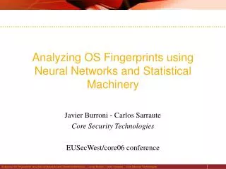
1. Using Neural Networks for remote OS Identification Javier Burroni - Carlos Sarraute Core Security Technologies PacSec/core05 conference

2. OUTLINE 1. Introduction2. DCE-RPC Endpoint mapper3. OS Detection based on Nmap signatures4. Dimension reduction and training

3. 1. Introduction2. DCE-RPC Endpoint mapper3. OS Detection based on Nmap signatures4. Dimension reduction and training

4. OS Identification • OS Identification = OS Detection = OS Fingerprinting • Crucial step of the penetration testing process • actively send test packets and study host response • First generation: analysis of differences between TCP/IP stack implementations • Next generation: analysis of application layer data (DCE RPC endpoints) • to refine detection of Windows versions / editions / service packs

5. Limitations of OS Fingerprinting tools • Some variation of “best fit” algorithm is used to analyze the information • will not work in non standard situations • inability to extract key elements • Our proposal: • focus on the technique used to analyze the data • we have developed tools using neural networks • successfully integrated into commercial software

6. 1. Introduction2. DCE-RPC Endpoint mapper3. OS Detection based on Nmap signatures4. Dimension reduction and training

7. Windows DCE-RPC service • By sending an RPC query to a host’s port 135 you can determine which services or programs are registered • Response includes: • UUID = universal unique identifier for each program • Annotated name • Protocol that each program uses • Network address that the program is bound to • Program’s endpoint

8. Endpoints for a Windows 2000 Professional edition service pack 0 • uuid="5A7B91F8-FF00-11D0-A9B2-00C04FB6E6FC" annotation="Messenger Service" • protocol="ncalrpc" endpoint="ntsvcs" id="msgsvc.1" • protocol="ncacn_np" endpoint="\PIPE\ntsvcs" id="msgsvc.2" • protocol="ncacn_np" endpoint="\PIPE\scerpc" id="msgsvc.3" • protocol="ncadg_ip_udp" id="msgsvc.4" • uuid="1FF70682-0A51-30E8-076D-740BE8CEE98B" • protocol="ncalrpc" endpoint="LRPC" id="mstask.1" • protocol="ncacn_ip_tcp" id="mstask.2" • uuid="378E52B0-C0A9-11CF-822D-00AA0051E40F" • protocol="ncalrpc" endpoint="LRPC" id="mstask.3" • protocol="ncacn_ip_tcp" id="mstask.4"

9. Neural networks come into play… • It’s possible to distinguish Windows versions, editions and service packs based on the combination of endpoints provided by DCE-RPC service • Idea: model the function which maps endpoints combinations to OS versions with a multilayer perceptron neural network • Several questions arise: • what kind of neural network do we use? • how are the neurons organized? • how do we map endpoints combinations to neural network inputs? • how do we train the network?

10. Multilayer Perceptron Neural Network 413 neurons 42 neurons 25 neurons

11. 3 layers topology • Input layer : 413 neurons • one neuron for each UUID • one neuron for each endpoint corresponding to the UUID • handle with flexibility the appearance of an unknown endpoint • Hidden neuron layer : 42 neurons • each neuron represents combinations of inputs • Output layer : 25 neurons • one neuron for each Windows version and edition • Windows 2000 professional edition • one neuron for each Windows version and service pack • Windows 2000 service pack 2 • errors in one dimension do not affect the other

12. What is a perceptron? • x1 … xn are the inputs of the neuron • wi,j,0 … wi,j,n are the weights • f is a non linear activation function • we use hyperbolic tangent tanh • vi,j is the output of the neuron Training of the network = finding the weights for each neuron

13. Back propagation • Training by back-propagation: • for the output layer • given an expected output y1 … ym • calculate an estimation of the error • this is propagated to the previous layers as:

14. New weights • The new weights, at time t+1, are: • where: learning rate momentum

15. Supervised training • We have a dataset with inputs and expected outputs • One generation: recalculate weights for each input / output pair • Complete training = 10350 generations • it takes 14 hours to train network (python code) • For each generation of the training process, inputs are reordered randomly (so the order does not affect training)

16. Sample result Neural Network Output (close to 1 is better): Windows NT4: 4.87480503763e-005 Editions: Enterprise Server: 0.00972694324639 Server: -0.00963500026763 Service Packs: 6: 0.00559659167371 6a: -0.00846224120952 Windows 2000: 0.996048928128 Editions: Server: 0.977780526016 Professional: 0.00868998746624 Advanced Server: -0.00564873813703 Service Packs: 4: -0.00505441088081 2: -0.00285674134367 3: -0.0093665583402 0: -0.00320117552666 1: 0.921351036343

17. Sample result (cont.) Windows 2003: 0.00302898647853 Editions: Web Edition: 0.00128127138728 Enterprise Edition: 0.00771786077082 Standard Edition: -0.0077145024893 Service Packs: 0: 0.000853988551952 Windows XP: 0.00605168045887 Editions: Professional: 0.00115635710749 Home: 0.000408057333416 Service Packs: 2: -0.00160404945542 0: 0.00216065240615 1: 0.000759109188052 Setting OS to Windows 2000 Server sp1 Setting architecture: i386

18. Result comparison • Results of our laboratory:

19. Introduction2. DCE-RPC Endpoint mapper3. OS Detection based onNmap signatures4. Dimension reduction and training

20. Nmap tests • Nmap is a network exploration tool and security scanner • includes OS detection based on the response of a host to 9 tests

21. Nmap signature database • Our method is based on the Nmap signature database • A signature is a set of rules describing how a specific version / edition of an OS responds to the tests. Example: # Linux 2.6.0-test5 x86 Fingerprint Linux 2.6.0-test5 x86 Class Linux | Linux | 2.6.X | general purpose TSeq(Class=RI%gcd=<6%SI=<2D3CFA0&>73C6B%IPID=Z%TS=1000HZ) T1(DF=Y%W=16A0%ACK=S++%Flags=AS%Ops=MNNTNW) T2(Resp=Y%DF=Y%W=0%ACK=S%Flags=AR%Ops=) T3(Resp=Y%DF=Y%W=16A0%ACK=S++%Flags=AS%Ops=MNNTNW) T4(DF=Y%W=0%ACK=O%Flags=R%Ops=) T5(DF=Y%W=0%ACK=S++%Flags=AR%Ops=) T6(DF=Y%W=0%ACK=O%Flags=R%Ops=) T7(DF=Y%W=0%ACK=S++%Flags=AR%Ops=) PU(DF=N%TOS=C0%IPLEN=164%RIPTL=148%RID=E%RIPCK=E%UCK=E%ULEN=134%DAT=E)

22. Wealth and weakness of Nmap • Nmap database contains 1464 signatures • Nmap works by comparing a host response to each signature in the database: • a score is assigned to each signature • score = number of matching rules / number of considered rules • “best fit” based on Hamming distance • Problem: improbable operating systems • generate less responses to the tests • and get a better score! • e.g. a Windows 2000 version detected as Atari 2600 or HPUX …

23. Hierarchical Network Structure • Analyze the responses with a neural network based function • OS detection is a step of the penetration test process • we only want to detect Windows, Linux, Solaris, OpenBSD, FreeBSD, NetBSD Windows DCE-RPC endpoint Linux kernel version relevant Solaris version OpenBSD version not relevant FreeBSD version NetBSD version

24. So we have 5 neural networks… • One neural network to decide if the OS is relevant / not relevant • One neural network to decide the OS family: • Windows, Linux, Solaris, OpenBSD, FreeBSD, NetBSD • One neural network to decide Linux version • One neural network to decide Solaris version • One neural network to decide OpenBSD version • Each neural network requires special topology design and training!

25. Neural Network inputs • Assign a set of inputs neurons for each test • Details for tests T1 … T7: • one neuron for ACK flag • one neuron for each response: S, S++, O • one neuron for DF flag • one neuron for response: yes/no • one neuron for Flags field • one neuron for each flag: ECE, URG, ACK, PSH, RST, SYN, FIN • 10 groups of 6 neurons for Options field • we activate one neuron in each group according to the option EOL, MAXSEG, NOP, TIMESTAMP, WINDOW, ECHOED • one neuron for W field (window size)

26. Example of neural network inputs • For flags or options: input is 1 or -1 (present or absent) • Others have numerical input • the W field (window size) • the GCD (greatest common divisor of initial sequence numbers) • Example of Linux 2.6.0 response: T3(Resp=Y%DF=Y%W=16A0%ACK=S++%Flags=AS%Ops=MNNTNW) • maps to:

27. Neural network topology • Input layer of 560 dimensions • lots of redundancy • gives flexibility when faced to unknown responses • but raises performance issues! • dimension reduction is necessary… • 4 layers neural network , for example the first neural network (relevant / not relevant filter) has: input layer : 204 neurons hidden layer1 : 96 neurons hidden layer2 : 20 neurons output layer : 1 neuron

28. Dataset generation • To train the neural network we need • inputs (host responses) • with corresponding outputs (host OS) • Signature database contains 1464 rules • a population of 15000 machines needed to train the network! • we don’t have access to such population… • scanning the Internet is not an option! • Generate inputs by Monte Carlo simulation • for each rule, generate inputs matching that rule • number of inputs depends on empirical distribution of OS • based on statistical surveys • when the rule specifies options or range of values • chose a value following uniform distribution

29. 1. Introduction2. DCE-RPC Endpoint mapper3. OS Detection based on Nmap signatures4. Dimension reduction and training

30. Inputs as random variables • We have been generous with the input • 560 dimensions, with redundancy • inputs dataset is very big • the training convergence is slow… • Consider each input dimension as a random variable Xi • input dimensions have different orders of magnitude • flags take 1/-1 values • the ISN (initial sequence number) is an integer • normalize the random variables: expected value standard deviation

31. Correlation matrix • We compute the correlation matrix R: • After normalization this is simply: • The correlation is a dimensionless measure of statistical dependence • closer to 1 or -1 indicates higher dependence • linear dependent columns of R indicate dependent variables • we keep one and eliminate the others • constants have zero variance and are also eliminated expected value

32. Principal Component Analysis (PCA) • Further reduction involves Principal Component Analysis (PCA) • Idea: compute a new basis (coordinates system) of the input space • the greatest variance of any projection of the dataset in a subspace of k dimensions • comes by projecting to the first k basis vectors • PCA algorithm: • compute eigenvectors and eigenvalues of R • sort by decreasing eigenvalue • keep first k vectors to project the data • parameter k chosen to keep 98% of total variance

33. Resulting neural network topology • After performing PCA we obtain the following neural network topologies (original input size was 560 in all cases)

34. Adaptive learning rate • Strategy to speed up training convergence • Calculate the quadratic error estimation ( yiare the expected outputs, vi are the actual outputs): • Between generations (after processing all dataset input/output pairs) • if error is smaller then increase learning rate • if error is bigger then decrease learning rate • Idea: move faster if we are in the correct direction

35. Error evolution (fixed learning rate) error number of generations

36. Error evolution (adaptive learning rate) error number of generations

37. Subset training • Another strategy to speed up training convergence • Train the network with several smaller datasets (subsets) • To estimate the error, we calculate a goodness of fit G • if the output is 0/1: G = 1 – ( Pr[false positive] + Pr[false negative] ) • other outputs: G = 1 – number of errors / number of outputs • Adaptive learning rate: • if goodness of fit G is higher, then increase the initial learning rate

38. Sample result (host running Solaris 8) • Relevant / not relevant analysis 0.99999999999999789 relevant • Operating System analysis    -0.99999999999999434 Linux 0.99999999921394744 Solaris    -0.99999999999998057 OpenBSD     -0.99999964651426454 FreeBSD     -1.0000000000000000 NetBSD     -1.0000000000000000 Windows • Solaris version analysis 0.98172780325074482 Solaris 8    -0.99281382458335776 Solaris 9     -0.99357586906143880 Solaris 7     -0.99988378968003799 Solaris 2.X     -0.99999999977837983 Solaris 2.5.X

39. Ideas for future work 1 • Analyze the key elements of the Nmap tests • given by the analysis of the final weights • given by Correlation matrix reduction • given by Principal Component Analysis • Optimize Nmap to generate less traffic • Add noise and firewall filtering • detect firewall presence • identify different firewalls • make more robust tests

40. Ideas for future work 2 • This analysis could be applied to other detection methods: • xprobe2 – Ofir Arkin, Fyodor & Meder Kydyraliev • detection by ICMP, SMB, SNMP • p0f (Passive OS Identification) – Michal Zalewski • OS detect by SUN RPC / Portmapper • Sun / Linux / other System V versions • MUA (Outlook / Thunderbird / etc) detection using Mail Headers

41. Questions?Thank you!