Image processing
Image processing. Reading. Jain, Kasturi, Schunck, Machine Vision . McGraw-Hill, 1995. Sections 4.2-4.4, 4.5(intro), 4.5.5, 4.5.6, 5.1-5.4. Image processing. An image processing operation typically defines a new image g in terms of an existing image f.


Image processing
E N D
Presentation Transcript
Reading • Jain, Kasturi, Schunck, Machine Vision. McGraw-Hill, 1995. Sections 4.2-4.4, 4.5(intro), 4.5.5, 4.5.6, 5.1-5.4. University of Texas at Austin CS384G - Computer Graphics Fall 2008 Don Fussell 2
Image processing • An image processing operation typically defines a new image g in terms of an existing image f. • The simplest operations are those that transform each pixel in isolation. These pixel-to-pixel operations can be written: • Examples: threshold, RGB grayscale • Note: a typical choice for mapping to grayscale is to apply the YIQ television matrix and keep the Y. University of Texas at Austin CS384G - Computer Graphics Fall 2008 Don Fussell 3
Pixel movement • Some operations preserve intensities, but move pixels around in the image • Examples: many amusing warps of images [Show image sequence.] University of Texas at Austin CS384G - Computer Graphics Fall 2008 Don Fussell 4
Noise • Image processing is also useful for noise reduction and edge enhancement. We will focus on these applications for the remainder of the lecture… • Common types of noise: • Salt and pepper noise: contains random occurrences of black and white pixels • Impulse noise: contains random occurrences of white pixels • Gaussian noise: variations in intensity drawn from a Gaussian normal distribution University of Texas at Austin CS384G - Computer Graphics Fall 2008 Don Fussell 5
Ideal noise reduction University of Texas at Austin CS384G - Computer Graphics Fall 2008 Don Fussell 6
Ideal noise reduction University of Texas at Austin CS384G - Computer Graphics Fall 2008 Don Fussell 7
Practical noise reduction • How can we “smooth” away noise in a single image? • Is there a more abstract way to represent this sort of operation? Of course there is! University of Texas at Austin CS384G - Computer Graphics Fall 2008 Don Fussell 8
Discrete convolution • For a digital signal, we define discrete convolution as: where University of Texas at Austin CS384G - Computer Graphics Fall 2008 Don Fussell 9
Discrete convolution in 2D • Similarly, discrete convolution in 2D becomes: where University of Texas at Austin CS384G - Computer Graphics Fall 2008 Don Fussell 10
Convolution representation • Since f and h are defined over finite regions, we can write them out in two-dimensional arrays: • Note: This is not matrix multiplication! • Q: What happens at the edges? University of Texas at Austin CS384G - Computer Graphics Fall 2008 Don Fussell 11
Mean filters • How can we represent our noise-reducing averaging filter as a convolution diagram (know as a mean filter)? University of Texas at Austin CS384G - Computer Graphics Fall 2008 Don Fussell 12
Effect of mean filters University of Texas at Austin CS384G - Computer Graphics Fall 2008 Don Fussell 13
Gaussian filters • Gaussian filters weigh pixels based on their distance from the center of the convolution filter. In particular: • This does a decent job of blurring noise while preserving features of the image. • What parameter controls the width of the Gaussian? • What happens to the image as the Gaussian filter kernel gets wider? • What is the constant C? What should we set it to? University of Texas at Austin CS384G - Computer Graphics Fall 2008 Don Fussell 14
Effect of Gaussian filters University of Texas at Austin CS384G - Computer Graphics Fall 2008 Don Fussell 15
Median filters • A median filter operates over an mxm region by selecting the median intensity in the region. • What advantage does a median filter have over a mean filter? • Is a median filter a kind of convolution? University of Texas at Austin CS384G - Computer Graphics Fall 2008 Don Fussell 16
Effect of median filters University of Texas at Austin CS384G - Computer Graphics Fall 2008 Don Fussell 17
Comparison: Gaussian noise University of Texas at Austin CS384G - Computer Graphics Fall 2008 Don Fussell 18
Comparison: salt and pepper noise University of Texas at Austin CS384G - Computer Graphics Fall 2008 Don Fussell 19
Edge detection • One of the most important uses of image processing is edge detection: • Really easy for humans • Really difficult for computers • Fundamental in computer vision • Important in many graphics applications University of Texas at Austin CS384G - Computer Graphics Fall 2008 Don Fussell 20
What is an edge? • Q: How might you detect an edge in 1D? University of Texas at Austin CS384G - Computer Graphics Fall 2008 Don Fussell 21
Gradients • The gradient is the 2D equivalent of the derivative: • Properties of the gradient • It’s a vector • Points in the direction of maximum increase of f • Magnitude is rate of increase • How can we approximate the gradient in a discrete image? University of Texas at Austin CS384G - Computer Graphics Fall 2008 Don Fussell 22
Less than ideal edges University of Texas at Austin CS384G - Computer Graphics Fall 2008 Don Fussell 23
Steps in edge detection • Edge detection algorithms typically proceed in three or four steps: • Filtering: cut down on noise • Enhancement: amplify the difference between edges and non-edges • Detection: use a threshold operation • Localization (optional): estimate geometry of edges beyond pixels University of Texas at Austin CS384G - Computer Graphics Fall 2008 Don Fussell 24
Edge enhancement • A popular gradient magnitude computation is the Sobel operator: • We can then compute the magnitude of the vector (sx, sy). University of Texas at Austin CS384G - Computer Graphics Fall 2008 Don Fussell 25
Results of Sobel edge detection University of Texas at Austin CS384G - Computer Graphics Fall 2008 Don Fussell 26
Second derivative operators • The Sobel operator can produce thick edges. Ideally, we’re looking for infinitely thin boundaries. • An alternative approach is to look for local extrema in the first derivative: places where the change in the gradient is highest. • Q: A peak in the first derivative corresponds to what in the second derivative? • Q: How might we write this as a convolution filter? University of Texas at Austin CS384G - Computer Graphics Fall 2008 Don Fussell 27
Localization with the Laplacian • An equivalent measure of the second derivative in 2D is the Laplacian: • Using the same arguments we used to compute the gradient filters, we can derive a Laplacian filter to be: • Zero crossings of this filter correspond to positions of maximum gradient. These zero crossings can be used to localize edges. University of Texas at Austin CS384G - Computer Graphics Fall 2008 Don Fussell 28
Localization with the Laplacian Original Smoothed Laplacian (+128) University of Texas at Austin CS384G - Computer Graphics Fall 2008 Don Fussell 29
Marching squares • We can convert these signed values into edge contours using a “marching squares” technique: University of Texas at Austin CS384G - Computer Graphics Fall 2008 Don Fussell 30
Sharpening with the Laplacian Laplacian (+128) Original Original + Laplacian Original - Laplacian Why does the sign make a difference? How can you write each filter that makes each bottom image? University of Texas at Austin CS384G - Computer Graphics Fall 2008 Don Fussell 31
Spectral impact of sharpening We can look at the impact of sharpening on the Fourier spectrum: Spatial domain Frequency domain University of Texas at Austin CS384G - Computer Graphics Fall 2008 Don Fussell 32
Summary • What you should take away from this lecture: • The meanings of all the boldfaced terms. • How noise reduction is done • How discrete convolution filtering works • The effect of mean, Gaussian, and median filters • What an image gradient is and how it can be computed • How edge detection is done • What the Laplacian image is and how it is used in either edge detection or image sharpening University of Texas at Austin CS384G - Computer Graphics Fall 2008 Don Fussell 33
Next time: Affine Transformations • Topic: • How do we represent the rotations, translations, etc. needed to build a complex scene from simpler objects? • Read: • Watt, Section 1.1.Optional: • Foley, et al, Chapter 5.1-5.5. • David F. Rogers and J. Alan Adams, Mathematical Elements for Computer Graphics, 2nd Ed., McGraw-Hill, New York, 1990, Chapter 2. University of Texas at Austin CS384G - Computer Graphics Fall 2008 Don Fussell 34