Modeling TCP Congestion Control
410 likes | 583 Vues
Modeling TCP Congestion Control. Don Towsley UMass Amherst towsley@cs.umass.edu. collaborators: T. Bu, W. Gong, C. Hollot, V. Misra. Outline. motivation TCP primer bottleneck invariance principle instability of RED active queue management

Modeling TCP Congestion Control
E N D
Presentation Transcript
Modeling TCP Congestion Control Don Towsley UMass Amherst towsley@cs.umass.edu collaborators: T. Bu, W. Gong, C. Hollot, V. Misra
Outline • motivation • TCP primer • bottleneck invariance principle • instability of RED active queue management • fixed point approximations of TCP networks • transient analysis of TCP networks • stochastic differential equations • summary
UDP-12Mbs TCP 12Mbs 1 B1=5Mbs 20Mbs 20Mbs B1= 2Mbs 2 { 1 B2=5Mbs 2 B2= 2Mbs 3 TCP B3=5Mbs 3 B3= 2Mbs 4 4 B4=5Mbs B4= 2Mbs Properties of TCP • 90% of Internet traffic • conservative end-end congestion control (CC) • equal bandwidth share • additive increase multiplicative decrease CC • only end-end protocol with congestion control TCP can be pushed around
Properties of TCP • 90% of Internet traffic • conservative end-end congestion control (CC) • equal bandwidth share • additive increase multiplicative decrease CC • only end-end protocol with congestion control Need to understand TCP in network setting
Additive-Increase Multiplicative-Decrease (AIMD) Congestion Control ri - rate after i-th feedback ri+1 = ri + c if i-th feedback is no congestion ri+1 = axriif i-th feedback indicates congestion, a<1 • similar algorithms for window-based CC • basic building block of most congestion control algorithms (e.g., TCP)
C . . . (r1,r2) ri2 C ri 1 AIMD and Fair Share • two sources, rates ri1,ri2 • bandwidth C • initial rates r1 and r2 • as time goes on, i increases, source rates converge to a fair share (Chiu,Jain 89)
Generic TCP Behavior • window algorithm (window W ) • up to W packets can be in network • return of ACK allows sender to send another packet • ACKS cumulative • increase window by one per RTT W <- W +1/W perACK W <- W +1 per RTT • seeks available network bandwidth
receiver W sender
Generic TCP Behavior • window algorithm (window W) • increase window by one per RTT W <- W +1/W per ACK • loss indication of congestion • decrease window by half on detection of loss (triple duplicate ACK), W <- W/2
receiver TD sender
Generic TCP Behavior • window algorithm (window W) • increase window by one per RTT W <- W +1/W per ACK • halve window on detection of loss, W <- W/2 • timeouts due to lack of ACKs -> window reduced to one, W <-1
receiver sender TO
Generic TCP Behavior • window algorithm (window W) • increase window by one per RTT (or one over window per ACK, W <- W +1/W) • halve window on detection of loss, W <- W/2 • timeouts due to lack of ACKs, W <-1 • successive timeout intervals grow exponentially long • slow start mechanism • provides fair share, full use of bandwidth
B(p,R) - TCP session throughput p - loss probability R - avg round trip time equilibrium analysis of AIMD B (p,R ) 1/R (1/p )1/2 • equilibrium analysis incl. timeouts (PFTK98) B (p,R ) [R (4p/3)1/2 + T0 3(3p/4)1/2p (1+32p 2)]-1 • T0 - timeout length Early Models
Experiments: 38 traces from 18 hosts unidirectional bulk transfers 100sec measurements Packets/s Measured PFTK p1/2 model Packets/s Measured PFTK p1/2 model Validation Observations: • many timeout loss events Conclusions: • good validation • other studies support model • insensitive to TCP version
Lessons • TCP exhibits well defined bandwidth curve • decreasing function of R and p • timeouts important • little difference between TCP versions • AIMD, timeouts • Vegas an exception
iBi(Ri ,p) = C Bottleneck invariance principle • bottleneck router • loss, high load, util. 1 • bottleneck invariance principle (BIP) C -router bandwidth Bi - throughput of flow i
Applications of BIP • provides simple checks of protocol design • active queue management, RED • new improved congestion control algorithms • accurate models of networks supporting infinite/finite duration TCP flows • thruput, loss rate, avg. queue length, …
Active queue management • drop tail - drop pkt when buffer fills • active queue management (AQM) • proactively drop/mark packets before buffer overflow • example: drop pkt with probability p(x) x - avg. queue length
- q (t ) -x (t ) x (t) : smoothed, time averaged q (t) x (ti +1) = aq (ti +d) + (1-a) x (ti) t RED (Random Early Detect) RED: marking/dropping based on average queue length x (t ) 1 marking prob p pmax tmin tmax 2tmax avg queue length x
C N N2 < N3 N3 < N4 N1 < N2 N1 N4 ? pmax N3 N2 N1 tmax RED discard function • RED queue • N identical TCP sources B(R,p) = C/N • p increases with N
C N pmax tmax RED discard function • RED queue • N identical TCP sources B(R,p) = C/N • p increases with N queue length N4 tmax
C N pmax tmax RED discard function • RED queue • N identical TCP sources B(R,p) = C/N • p increases with N • once p > pmax, queue oscillates around tmax RED unstable! (Firoiu, Borden, 00)
Improved RED 1 discontinuity removed in gentle_ variant Marking prob. p pmax tmin tmax 2tmax Avg queue length x
1 N • N infinite sourceTCP sessions B (p(q ), R (q )) = C /N Stationary Behavior: single bottleneck • one bottleneck link • AQM; avg. queue length q, discard prob. p(q) • bandwidth C • R (q) = R0 + q /C (round trip time)
Single bottleneck • solve a fixed point problem for q • unique solution provided B is monotonic and continuous • resulting q can be used to obtain Ri and p • preliminary evaluation results good
PFKT Model p1/2 Model Simulation + RT Model p1/2 Model Results: single Bottleneck • N TCP flows • two-way prop. delay • 18+2i ms, i = 1,…,N • link bandwidth N • RED: scaled by N similar results for short-lived flows
N TCP flows throughputs {Bi} V congested RED routers capacities {Cv } avg. queue lengths x = {xv } discard prob. p = {pv (xv )} TCP model: Bi(R , p) congested router model iBi(x) = Cv , v =1,…,V V equations, V unknowns Network Setting TCP flow Bi AQM router Cv, pv(xv)
RT Model p1/2 Model + Estimated end to end loss Measured end2end loss Results: Tandem Networks • 8networks, 5 -10routers • 2-way propagation delay20-120ms • bandwidth, 2-6 Mbps • error • throughput < 10% • loss rate < 10% • avg. queue length < 15% • similar results for cyclic networks
1 N Transient Analysis: single router • one congested router • capacity {C (packets/sec)} • queue length q (t ) • discard prob. p(t ) • N TCP flows • window sizes Wi (t ) • round trip time Ri(t ) = Ai +q (t )/C • throughputs Bi(t ) = Wi (t )/Ri (t )
= dt - Wi dNi (t-t) Ri (q (t)) 2 Additive increase Mult. decrease System of Stochastic Differential Equations Assumption: Poisson loss process{Ni (t)}: Window Size: dWi {Ni (t)}: time varying, rate Wi (t ) p (x (t )) / Ri (q (t)) t : feedback delay (round trip time) Timeouts ignored
dt Wi dNi (t-t) Ri (q (t)) 2 = - 1{q (t) > 0}C dt dt Wi (t ) + S Outgoing traffic Incoming traffic Ri (q (t )) System of SDEs Window Size: dWi = - Queue length: dq
EWi 2 dEWi dt - EWi(t-t) Queue length: dEq dt -1{Eq(t) > 0}C + S Ri(Eq(t)) Ri (Eq(t-t)) EWi(t) System of Differential Equations 1 Ep(t-t) Window Size: Ri(Eq(t)) Conjecture: exact as no. flows ->
ln (1-a) ln (1-a) d d dEp dt dp dx dEx dt = Loss probability: Eq(t) p x System of Differential Equations (cont.) Estimated average queue length: dEx dt Ex(t) = - a = averaging parameter of RED d = sampling interval ~ 1/C dp/dx is obtained from the marking profile
dEp dt = f3(Eq) dEq dt = f2(EWi) Result: N +2 coupled equations dEWi dt = f1(Ep,Ri, EWi) i = 1..N Numerical solution using MATLAB
Queuing delay- aggregate delay q(t )=SV qV(t ) loss probability- cumulative loss probability p(t)= 1-PV (1-pV(t )) Extension to Network Networked case:V congested AQM routers Other extensions to model Timeouts:leveraged work done in [PFTK Sigcomm98] to model timeouts Flow aggregation:represent flows sharing same route by single equation
Flow set 4 Flow set 1 RED router 1 Flow set 2 Flow set 3 Flow set 5 Validation scenario Topology • two RED routers • one way ftp flows traffic sources • comparison to ns • transient queuing performance obtained RED router 2 5 sets of flows 2 RED routers Set 2 flows through both routers
Fluid model ns simulation Performance of DE method • link rates 5 Mb/s • load variation at t=75 and t=150 seconds • 200 flows simulated • drops to 120 between t = 75, 120 • fluid model captures transient performance Inst. Queue length Time
Observations on RED • “Tuning” of RED is difficult - sensitive to packet sizes, load levels, round trip time, etc. • oscillations due to • exponential smoothing of queue length • use of variable sampling interval d • feedback delay • queue fill delay Further Work Detailed Control Theoretic Analysis of TCP/REDavailable at http://gaia.cs.umass.edu/papers/papers.html
Improving congestion control Working with linearized model • developed rules for setting RED parameters • compared Proportional Integral (PI) controller with properly adjusted RED • ns simulation with time varying http,ftp flows • PI controller: faster response, decouples queue size and load level Queue length vs. Time - PI Controller - RED Controller queue length time
Conclusions • fixed point approach promising for stationary behavior of TCP • DE approach promising for more detailed transient behavior • computation cost of methods a fraction of the discrete event simulation cost • formal representation and analysis yields better understanding of RED/AQM