Experimental Fluid Dynamics and Uncertainty Assessment Methodology
350 likes | 478 Vues
This document presents a detailed methodology for Experimental Fluid Dynamics (EFD), focusing on the use of experimental techniques in fluid engineering. It covers the philosophy and processes of EFD, including test setups, data acquisition, data reduction, and uncertainty analysis. The objective is to facilitate better understanding and validation of fluid dynamics theories while providing essential benchmarking data for industry applications. Key instruments, methodologies, and practical setups are discussed, contributing to advancements in research, development, and educational purposes.

Experimental Fluid Dynamics and Uncertainty Assessment Methodology
E N D
Presentation Transcript
Experimental Fluid Dynamics and Uncertainty Assessment Methodology H. Elshiekh, H. Yoon, M. Muste, F. Stern Acknowledgements: S. Ghosh, M. Marquardt, S. Cook
Table of Contents • What is EFD • EFD philosophy • EFD Process • Test Setup • Data Acquisition • Data Reduction • Uncertainty analysis • Data Analysis • 57:020 EFD Labs
1. What is EFD Experimental Fluid Dynamics (EFD): Use of experimental methodology and procedures for solving fluids engineering systems, including full and model scales, large and table top facilities, measurement systems (instrumentation, data acquisition and data reduction), dimensional analysis and similarity and uncertainty analysis. Purpose: • Science & Technology: understand and investigate a phenomenon/process, substantiate and validate a theory (hypothesis) • Research & Development: document a process/system, provide benchmark data (standard procedures, validations), calibrate instruments, equipment, and facilities • Industry: design optimization and analysis, provide data for direct use, product liability, and acceptance • Teaching: Instruction/demonstration A pretty experiment is in itself often more valuable than twenty formulae extracted from our minds." - Albert Einstein
2. EFD Philosophy • Decisions on conducting experiments are governed by the ability of the expected test outcome to achievethe experimentobjectives within allowable uncertainties. • Integration of UA into all test phases should be a key part of entire experimental program • test design • determination of error sources • estimation of uncertainty • documentation of the results
3. EFD Process • EFD labs provide “hands on” experience with modern measurement systems, understanding and implementation of EFD in practical application and focus on “EFD process”:
1) Test Setup • Types of measurements and instrumentation
Manometers • Principle of operation:Manometers are devices in which columns of suitable liquid are used to measure the difference in pressure between two points, or between a certain point and the atmosphere (patm). • Applying fundamental equations of hydrostatics the pressure difference, P, between the two liquid columns can be calculated. • Manometers are frequently used to measure pressure differences sensed by Pitot tubes to determine velocities in various flows. • Types of manometers: simple, differential (U-tube), inclined tube, high precision (Rouse manometer). U-tube manometer
Pressure transducers A pressure transducer converts the pressure sensed by the instrument probe into mechanical or electrical signals Pressure transducer Elastic elements used to convert pressure within transducers Transducer read out
Pressure transducers Schematic of a membrane-based pressure transducer • A a diaphragm separates the high and low incoming pressures. • The diaphragm deflects under the pressure differencethus changing the capacitance(C) of the circuit, which eventually changes the voltage output(E). • The voltages are converted through calibrations to pressure units. • Pressure transducers are used with pressure taps, pitot tubes, pulmonary functions, HVAC, mechanical pressures, etc.
Pressure taps • Static(Pstat) and stagnation(Pstag) pressures • Pressure caused only by molecular collisions is known as static pressure. • The pressure tap is a small opening in the wall of a a duct (Fig a.) • Pressure tap connected to any pressure measuring device indicates the static pressure. (note: there is no component of velocity along the tap axis). • The stagnation pressure at a point in a fluid flow is the pressure that could result if the fluid was brought to rest isentropically (i.e., the entire kinetic energy of the fluid is utilized to increase its pressure only). Single and multi pressure taps
Pitot tube • The tubes sensing static and stagnation pressures are usually combined into one instrument known as pitot static tube. • Pressure taps sensing static pressure (also the reference pressure for this measurement) are placed radially on the probe stem and then combined into one tube leading to the differential manometer (pstat). • The pressure tap located at the probe tip senses the stagnation pressure (p0). • Use of the two measured pressures in the Bernoulli equation allows to determine one component of the flow velocity at the probe location. • Special arrangements of the pressure taps (Three-hole, Five-hole, seven-hole Pitot) in conjunction with special calibrations are used two measure all velocity components. • It is difficult to measure stagnation pressure in real, due to friction. The measured stagnation pressure is always less than the actual one. This is taken care of by an empirical factor C. P0 = stagnation pressure Pstat = static pressure
Venturi meter • Venturi meter consists of two conical pipes. The minimum cross section diameter is called throat. The angles of the conical pipes are established to limit the energy losses due to flow separation. • The flow obstruction produced by the venturi meter produces a local loss that is proportional to the flow discharge. • Pressure taps are located upstream and downstream of venturimeter, immediately outside the variable diameter areas, to measure the losses produced through the meter. • Flow rateis calculated using Bernoulli equation and the continuity equation. An experimental coefficient is used to account for the losses occurring in the meter (Va and Vb are the upstream and downstream velocities and r is the density. (Aa and Ab are the cross sectional areas).
Hotwire • Single hot-wire probe • Platinum plated Tungsten • 5 m diameter, 1.2 mm length • Constant temperature anemometer • Used for mean and instantaneous (fluctuating) velocity measurements • Principle of operation: Sensor resistance is changed by the flow over the probe and the cooling taking place is related through calibration to the velocity of the incoming flow. • The tool is very reliable for the measurement of velocity fluctuations due to its high sampling frequency and small size of the probe. • Cross-wire (X) probe • Two sensors perpendicular to each other • Measures within 45
Loadcell Principle • Load cells measure forces and moments by sensing the deformation of elastic elements such as springs. • Usually it comprises of two parts • the spring: deforms under the load (usually made of steel) • sensing element: measures the deformation (usually a strain gauge glued to the deforming element). • Load cell measurement accuracy is limited by hysteresis and creep, that can be minimized by using high-grade steel and labor intensive fabrication.
Particle Image Velocimetry (PIV) • PIV setup • Images of the flow field are captured with camera(s). • 1 camera is used for 2-dimesional flow field measurement • 2 cameras are used for stereoscopic 2-dimesional measurement, whereby a third dimension can be extracted → 3-dimensional • 3 or more cameras are used for 3-dimensional measurement • Illumination comes from laser(s), LED’s, or other lights sources • Fluid is saturated with small and neutrally buoyant particles
Particle Image Velocimetry (PIV) • Principle of PIV operation • Particles in flow scatter laser(s) light • Two images, per camera, are taken within a small time of one another Δt. • Both images are divided into identical smaller sections, called interrogation windows • Patterns of particles within an interrogation window are traced • Image pixels are calibrated to a known distance • Number of pixels between a particle and the same particle Δt later == a distance • →process called cross correlation • Velocity = direction × (distance a particle travels/ Δt)
Particle Image Velocimetry (PIV) • Advantages of PIV • Entire velocity field can be calculated • Capability of measuring flows in 3-D space • Generally, the equipment is nonintrusive to flow • High degree of accuracy • Disadvantages of PIV • Requires proper selection of particles • Size of flow structures are limited by resolution of image • Costly
2) Data acquisition - Outline • General scheme of a data acquisition: • Special considerations: • Correlate sampling type, sampling frequency (Nyquist criterion), and sampling time with the dynamic content of the signal andthe flow nature (laminar or turbulent) • Correlate the resolution for the A/D converters with the magnitude of the signal • Identify sources of errors for each step of signal conversion
2) Data acquisition - hardware Adapter cable 8 port smart switch RS232 PCI serial card 8 – channel analog input module Computerized automated data acquisition system
2) Data Acquisition - Software • Introduction to Labview • Labviewis a programming software used for data acquisition, instrument control, measurement analysis, and more. • Graphical programming language that uses icons instead of text. • Labviewallows to build user interfaces with a set of tools and objects. • The program is written on block diagrams and a front panel is used to control and run the program. Typical Labviewfron-panel interface
3) Data Reduction • A step to convert massive raw data into meaningful results • Done by: • Performing statistical analysis (e.g. mean and standard deviation) • Applying data reduction equations • Data reduction equations represents the experiments targeted variable as a function of the measured variables (, , … ,) e.g.) Kinematic viscosity, :
4) Uncertainty Analysis • Uncertainty analysis (UA) is a rigorous methodology for uncertainty assessment using statistical and engineering concepts • ASME and AIAA standards (e.g., ASME, 1998; AIAA, 1995) and ISO Guide (1995) are the most commonly used of UA methodologies, which are internationally recognized • More recent standard ASME (2005) is a revision of ASME (1998) for a better harmonization with the ISO Guide (1995)
4) Uncertainty Analysis Definitions: • Error: Difference between measured and true value • Uncertainty: Estimate of errors in measurements of individual variables or results • Estimates of uncertainty is usually made at 95% confidence level Note: • Accuracy: Closeness of agreement between measured and true value
4) Uncertainty Analysis Error sources: Uncertainty limits:
4) Uncertainty Analysis Error propagation:Block diagram shows identifications of elemental error sources for individual measurement system or individual measurement variables and their propagation through data reduction equations and to the final experimental results
5) Data Analysis • Data analysis • Curve fitting techniques • Statistical techniques • Spectral analysis (Fast Fourier Transform) • Proper orthogonal decomposition • Data visualizations • Comparisons of the results with bench mark data, CFD, and/or AFD • Evaluate fluid physics • Prepare report
4. 57:020 EFD Labs • Three EFD labs • Each lab consists of two parts: EFD General and ePIV • Total 6 lab activities
1) Lab 1 – Viscosity experiment • Kinematic viscosity and mass density measurements for Glycerin: • Definition of “EFD Process” • Data reduction equation • Estimates of errors and uncertainties • Bias, precision, and total uncertainty
2) Lab 1 – Cylinder flow (ePIV) • Flow streamline visualization around a circular cylinder model • PIV camera settings • Flow streamlines visualization around bluff bodies
3) Lab 2 – Pipe experiment • Flow rate, friction factor, and velocity profile measurements for smooth and rough pipes • Comparison between automated and manual data acquisition systems • Measurement systems using pressure tap, Venturi-meter, and pitot probe • Automated data acquisition using LabView • The importance of non-dimensionalization and comparison of results with benchmark data
4) Lab 2 – Step-up flow (ePIV) • Flow rate and average velocity for a step-up model • PIV image correlation parameters and PIV data reduction • Mass conservation law (flow rate and average velocity)
5) Lab 3 – Airfoil experiment • Surface pressure distribution, wake velocity profile, and lift and drag forces measurements for a Clark-Y airfoil model • Using LabView for setting test conditions and data acquisition • Calibration of loadcell • Measurement of lift and drag forces with loadcell • Measurement of pressure distribution and velocity profile for an airfoil model
6) Lab 3 – Airfoil flow (ePIV) • Velocity field and flow streamlines around Clark-Y airfoil model (miniature) • PIV data post-processing using Tecplot software • Flow around lifting bodies
Lab Schedule and Report Instructions • Lab Schedule: See the class website: http://css.engineering.uiowa.edu/~fluids/fluids.htm • Lab report instructions See the class website: http://css.engineering.uiowa.edu/~fluids/documents/ instructions_for_lab_report.pdf