Optical Switching Networks
Optical Switching Networks. Presentation by Joaquin Carbonara. References. Work by Ngo,Qiao,Pan, Anand, Yang Chu/Liu/Zhang Pippinger/Feldman/Friedman Winkler/Haxell/Rasala/Wilfong. Introduction. Statement of the Problem. About Optical Networks.

Optical Switching Networks
E N D
Presentation Transcript
Optical Switching Networks Presentation by Joaquin Carbonara
References • Work by • Ngo,Qiao,Pan, Anand, Yang • Chu/Liu/Zhang • Pippinger/Feldman/Friedman • Winkler/Haxell/Rasala/Wilfong
Introduction Statement of the Problem
About Optical Networks • Wavelength-routed all-optical WDM networks are considered to be candidates for the next generation wide-area Backbone networks [Chlamtac,Ganz and Karmi, 1992 and Mukherjee, 2000] • Wavelength Routed Network: wavelength routers connected by fiber links (each being able to support wavelength channels by supporting WDM) • WXC can be uni/multicast. OXC can be used between processors in a parallel or distributed system.
About Optical networks • In a dynamic wavelength-routed WDM network, limitations of the network may result in some light-paths requests not being satisfied. • Goal: design all-optical networks that minimizes blocking.
About Optical Networks • Wavelength Continuity Constraint (which makes Optical nets different than circuit-switched telephone nets):Thustwo light paths that share a common fiber link should not be assigned the same wavelength. • Solution: Wavelength converters.
About Optical Networks • Switching speed is the bottleneck at the core of the optical network infrastructure [Singhal and Jain, 2002] • Goal: design cost-effective WXC that are fast and easily scalable.
Design analysis • RNB (rearrangeable non-blocking): a set of requests submitted at once can be satisfied by the network. • SNB (Strictly non-blocking): a new request can be satisfied without changing current request paths. • WSNB (Wide sense non-blocking): a new request can be satisfied using an (on-line) algorithm. • SNB --> WSNO --> RNB
Design Analysis • Cost of components is important. • Number of different components: • (de)multiplexors (MUX/DEMUX) • Wavelenght converters (full-FWC or limited-LWC) • Semiconductor Optical Amplifiers (SOA) • Optical add-drop multiplexors (OADM) • Arrayed Waveguide Grating Routers (AWGR)
Design Analysis • Theoretical results help understand and design networks • Complexity is important (as a function of size) • Size: number of edges in graph theoretical representation • Depth: number of edges in longest path of graph theoretical representation.
Design tools • Mathematical modeling • Graph Theory; Theory of Discrete Mathematics/Combinatorics; Functions (Real/Integer valued, one or more variables); Linear/Multilinear Algebra. • In mathematics you don't understand things. You just get used to them. von Neumann, Johann (1903 - 1957) • Mathematicians are a species of Frenchmen: if you say something to them they translate it into their own language and presto! it is something entirely different. Goethe (German writer), Maxims and Reflexions, (1829)
Design tools • Advantages of mathematical modeling: • Many tools available since Mathematics is an old and well established discipline • True statements are backed by proofs (100% guaranteed--if used properly). • Math language is practically universal. This guarantees a larger audience . • Math organizes knowledge extremely well.
Design tools • Disadvantages of Mathematical modeling • It is hard to fit reality into a “nice” Theory • Theory requires organized abstract thinking--not a very popular activity
Design Tools • Other tools include simulation and analysis (I will not talk about these tools).
Optical Network Design Definitions, Examples and Theoretical Results
Components: Wavelength Converters • Wavelength converters: take as input wavelengths coming on different fibers and can be programmed to modify the wavelength and output modified wavelength. • To reduce cost, researchers have • Used Limited Range Wavelength converters (LWC) instead of Full Range Wavelength converters (FWC) • Share wavelength converters among fiber links. • Notation: LWC(A,B) takes inputs from set A and produces outputs from set B.
Components:AWGR • Arrayed Waveguide Grating Routers: • Passive devices: reroute channels inside fibers • Easily available and inexpensive • Take m inputs and have m outputs fibers • Process wavelengths 0 to m-1 • Wavelength i at input fiber j gets routed to the same wavelength at output fiber (i-j)mod m.
Request Model(understanding Nets blocking properties) • Model 1 -- (, F, F): Requests are of the form (i, Fj, Fj ) where i is a wavelength, Fj is an input fiber and Fj is an output fiber. Requests requires only an given output fiber, but do not specify the output wavelength. • Model 2 -- (, F, , F): More restrictive than Model 1 since output wavelength is also requested. • Note: If N satisfies M2 then it satisfies M1
WXC-RNB construction for M1(Ngo/Pan/Qiao infocom ‘04) • Components: Let f=2, b=3, n=4. Then it has f demultx, fbn LWC(Bi,[n]), fbn n-AWG, fbn LWC([n],[bc,b(f+c)]), n multx, nb nb-AWG, and f multx.
WXC-RNB-1 means ... • RNB means that any set S of valid requests will not be blocked in the network N. While in transit inside the network, the Wavelength Continuity Constrain must be satisfied. • Valid request means • no two requests will ask for the same input wavelength and fiber. • the number of requests asking for the same output fiber cannot exceed the fiber capacity.
WXC-RNB-1 and GT • Konig’s 1916 Theorem: Let G(U,V;E) be a bipartite graph. Then: the maximum (vertex) degree equals the chromatic index. • Chromatic index= minimum number of colors needed to edge color G so that adjacent edges use different colors.
Back to WXC-RNB-1... • Represent the network as a bipartite graph G(U,V;E) for the sole purpose of determining a non-blocking route for each request: • The set U corresponds to the set of input bands (there are fb of them) • The set V corresponds to the set of output fibers (there are f of them)
Graph of WXC-RNB-1 • Represent the network as a bipartite graph G(U,V;E): • Request (p, Fq, Fj) edge (ui,vj) where i = qb+ p/n • By a simple variation of Konig’s theorem, the graph G is colorable with n x b colors (label each color with a tuple (c,d)), 1≤c ≤n and 1≤d ≤b, in such a way that edges sharing a vertex in U have different first color component.
Routing in WXC-RNB-1 • The basic idea is this: 1. [request (p, Fq, Fj)] [edge (ui,vj)] [color (c,d)] 2. Then Route p so that it ends up in the cthoutput line of its stage-1 AWGR. 3. Working from the other end, we want the request to end in Fj. There are b fibers demuxing to it. We can see that if the stage-2 LWC routes the wavelength to its dth line of its demuxer, the desired output is obtained.
Routing in WXC-RNB-1 • The basic idea is this (cont.): 4. The properties of the coloring inherited from Konig’s theorem guaranteed non-blockiness.
Other interesting results related to non-blocking networks • Strictly non-blocking networks are highly desirable. It is difficult to build such networks that are cost efficient. • An interesting result (Ngo): WXC-SNB-1 if and only if WXC-SNB-2
Optical Network Complexity Graph Theoretical representations, Bounds, minimizing the number of components. Examples and theoretical results.
Complexity: Minimizing the Number of LWC • Results related to using the least possible number of LWC on a uni/multicast network: • Define LWC(d) when LWC can convert i to j iff |i-j|≤d. • Consider Homogenous Model-2 of requests with w wavelengths and f fibers (HM2(w, f)). • Want to study statistic m1(w,f,d) = least number of LWC(d) needed if HM2(w, f) is SNB.
Complexity of WDM networks(unicast) m1(w,f,d) even w (Ngo/Pan/Yang)
Complexity of WDM networks (unicast) m1(w,f,d) odd w (Ngo/Pan/Yang)
Complexity: Size and Depth using GT representation • (Ngo) Using the DAG model (Directed Acyclic Graphs) we can establish a formal definition of size and depth of a network. • Size: number of edges in the graph • Depth: number of edges in the longest path.
ComplexityUsingGraph/Theoretical Representation • (Ngo) Graph Theoretical representation. • a) Fiber-channels get replaced by vertices • b) Edges ~ capacity
ComplexityUsingGraph/Theoretical RepresentationExample • Size of the network is number of edges. • Depth is longest path. • It uses 2 2x2 AWG, 4 FWC 2 multiplexors and 2 demultiplexors • DAG=Directed Acyclic Graph
Graph/Theoretical Representation(Winkler/Haxell/Rasala/Wilfong)Dynamic bipartite graphs
ComplexityUsingDAG GT RepresentationRigorous Setting Model-2 • DAG model networks as follows: • (n1,n2)-network is a DAG N=(V,E;A,B) V=vertices, E=edges, A=inputs, B=outputs, n1= |A|, n2=|B|. • We can now define request, request frame, route, RNB/SNB/WSNB network. • Key idea: requests’ path must be disjoint to be (simultaneously) realizable.
ComplexityUsingGraph/Theoretical RepresentationRigorous Setting Model-1 • DAG model networks as follows: • [w,f]-network is a DAG N=(V,E;A,B) V=vertices, E=edges, A=inputs, B=outputs |A|=|B|=wf and B=B1 B2 ... Bf • We can now define request, request frame, route, and RNB/SNB/WSNB [w,f]-network.
Complexity: DAG size • Let an n-network be a Homogeneous Network with n inputs and outputs. If the output is further divided into f bands of size w (needed for M-2) we call it a [w,f]-network. • The smallest number of edges (size) for it to be SNB, RNB, and WSNB is sc2(w,f), rc2(w,f) and wc2(w,f) (Model 2), or sc1(n), rc1(n) and wc1(n) (Model 2). • rc1(n)≤wc1(n) ≤ sc1(n),
Complexity:Results from DAG model • M1 is less restrictive than M2 since M2 requests specify an output wavelength. The following result shows that in the SNB case there is no difference in cost between models:
Complexity:RNB [w,f]-networks • The size function has known estimates in this case:
Complexity • Advantages of having bounds: • Number of edges can be related to network cost • Theoretical results are often the only way to gain experience with abstract systems. Examples may be too poor or difficult to concoct.
Complexity • Other results include different ways of create “atomic” networks, and operations to create larger networks from smalles • Left and right union • The -product
Future Work • Expansion of current models using different models with the goal of eliminating blockiness while reducing cost. • Search for better bounds on the current statistics. • Search for new meaningful statistics (is size and depth the only ones that matter?) on GT representations.