Download
1 / 53
540 likes | 654 Vues
The Costs of Production Principles of Microeconomics Boris Nikolaev. Brainstorming costs. You run Ford Motor Company. List three different costs you have. List three different business decisions that are affected by your costs. In this chapter.

E N D
The Costs of ProductionPrinciples of Microeconomics Boris Nikolaev
Brainstorming costs You run Ford Motor Company. • List three different costs you have. • List three different business decisions that are affected by your costs.
In this chapter • What is a production function? What is marginal product? How are they related? • What are the various costs? How are they related to each other and to output? • How are costs different in the short run vs. the long run? • What are “economies of scale”?
It’s business time. • Firms are in the business of making profits. Profit = Total Revenue (TR) – Total Cost (TC) the market value of the inputs a firm uses in production the amount a firm receives from the sale of its output
Sneak Preview MR=MC
Profits • Are profits bad? • What is the function of profits in a free market economy? • In a competitive market profits come not from increase in price, but from decrease in the cost of production. Why? • Fortune 500 most profitablecompanies [see here]
Profits and Insurance • Recollect risk-aversion & uncertainty.
Marxist View • The stagnating wages since the 1970s • Technology • World war II • Outsourcing • Women in the labor force • Immigration • Problem of effective demand • Work more hours • Borrowing binge (mortgage debt, credit cards) • Greatest profit boom (in the history of the world) • Marginal productivity, wages, and profits
What do you do with the profits? • CEO salaries [Forbes list] • Mergers & Acquisitions • Lend to employees (e.g. GM, IBM, etc.)
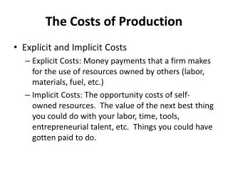
Costs • Resources are scarce, productive, and have alternative uses. Explicit costs are the direct cash payments you make to use resources you don’t own such as wages, rent, insurance, taxes, etc. Implicit costs is the opportunity cost of the resource you own (the benefit you could have extracted from it from its next best use). Do not require direct cast payments.
Example You need $100,000 to start your business. The interest rate is 5%. • Case 1: borrow $100,000 • explicit cost = $5000 interest on loan • Case 2: use $40,000 of your savings, borrow the other $60,000 • explicit cost = $3000 (5%) interest on the loan • implicit cost = $2000 (5%) foregone interest you could have earned on your $40,000.
Economic vs Accounting Profit • Accounting profit = total revenue minus total explicit costs • Economic profit = total revenue minus total costs (including explicit and implicit costs) • Accounting profit ignores implicit costs, so it’s higher than economic profit.
Example 1 The equilibrium rent on office space has just increased by $500/month. Determine the effects on accounting profit and economic profit if: a.you rent your office space b.you own your office space
Answers The rent on office space increases $500/month. a.You rent your office space. Explicit costs increase $500/month. Accounting profit & economic profit each fall $500/month. b. You own your office space. Explicit costs do not change, so accounting profit does not change. Implicit costs increase $500/month (opp. cost of using your space instead of renting it) so economic profit falls by $500/month.
Practice Question Your current job pays $50K/year. You have $20K savings that earn you $3K interest a year. You own a garage, which you rent for $12K/ year. You decide to invest your savings and use your garage to start your own business. Did you make a good economic decision? Total Revenue $105K Explicit Costs labor $21K food $20K Total Cost $41K Accounting Profit _____ Implicit Costs salary _____ interest _____ rent _____ Total Implicit Cost _____ Economic Profit / Loss ______
Production in the Short Run Q= f(L,K) A production function shows the relationship between the quantity of inputs used to produce a good and the quantity of output of that good.
EXAMPLE 1: Production Function L(no. of workers) Q(bushels of wheat) 3,000 2,500 0 0 2,000 1 1000 1,500 Quantity of output 2 1800 1,000 3 2400 500 4 2800 0 0 1 2 3 4 5 5 3000 No. of workers 0
Marginal Product (MP) If you hire one more worker, your output rises by the marginal product of labor. The marginal productof any input is the increase in output arising from an additional unit of that input, holding all other inputs constant. Notation: ∆ (delta) = “change in…” Examples: ∆Q = change in output, ∆L = change in labor Marginal product of labor (MPL) = ∆Q ∆L 0
EXAMPLE 1: Total & Marginal Product L(no. of workers) Q(bushels of wheat) 0 0 ∆Q = 1000 ∆L = 1 1 1000 ∆Q = 800 ∆L = 1 2 1800 ∆L = 1 ∆Q = 600 3 2400 ∆Q = 400 ∆L = 1 4 2800 ∆L = 1 ∆Q = 200 5 3000 0 MPL 1000 800 600 400 200
EXAMPLE 1: MPL = Slope of Prod Function 3,000 2,500 2,000 Quantity of output 1,500 1,000 500 0 0 1 2 3 4 5 No. of workers 0 L(no. of workers) Q(bushels of wheat) MPL MPL equals the slope of the production function. Notice that MPL diminishes as L increases. This explains why the production function gets flatter as L increases. 0 0 1000 1 1000 800 2 1800 600 3 2400 400 4 2800 200 5 3000
Why MPL Is Important • Recall one of the Ten Principles:Rational people think at the margin. • When you hire an extra worker, • your costs rise by the wage he pays the worker • your output rises by MPL • Comparing them helps you decide whether he should hire the worker.
The Law of Diminishing Marginal Returns • Diminishing marginal product: The marginal product of an input declines as the quantity of the input increases (other things equal). • Why does it decline?
Practice Question Assume that only one input (L) is relevant in production. The wage / worker = $175 and one pound of fish is selling for $10
Let’s go back to our farm example… • You must pay $1000 per month for the land, regardless of how much wheat you grow. • The market wage for a farm worker is $2000 per month. • Your cots are related to how much wheat you produce…
EXAMPLE 1: Your Costs $1,000 $0 $1,000 $1,000 $2,000 $3,000 $1,000 $4,000 $5,000 $1,000 $6,000 $7,000 $1,000 $8,000 $9,000 $1,000 $10,000 $11,000 0 L(no. of workers) Q(bushels of wheat) Cost of land Cost of labor Total cost 0 0 1 1000 2 1800 3 2400 4 2800 5 3000
Marginal Cost Marginal Cost (MC) is the increase in Total Cost from producing one more unit: MC = ∆TC ∆Q
EXAMPLE 1: Total and Marginal Cost Q(bushels of wheat) Total Cost 0 $1,000 ∆TC = $2000 ∆Q = 1000 1000 $3,000 ∆TC = $2000 ∆Q = 800 1800 $5,000 ∆TC = $2000 ∆Q = 600 2400 $7,000 ∆TC = $2000 ∆Q = 400 2800 $9,000 ∆TC = $2000 ∆Q = 200 3000 $11,000 Marginal Cost (MC) $2.00 $2.50 $3.33 $5.00 $10.00
EXAMPLE 1: The Marginal Cost Curve $2.00 $2.50 $3.33 $5.00 $10.00 Q(bushels of wheat) TC MC MC usually rises as Q rises, as in this example. 0 $1,000 1000 $3,000 1800 $5,000 2400 $7,000 2800 $9,000 3000 $11,000
Why MC Is Important • You are rational and want to maximize your profits. To increase profit, should you produce more or less wheat? • To find the answer, you need to “think at the margin.” • If MC > MR then producing one more unit will decrease profits.
0 Fixed and Variable Costs • Fixed costs(FC) do not vary with the quantity of output produced. • In our example, FC = $1000 for land • Other examples: cost of equipment, loan payments, rent • Variable costs (VC) vary with the quantity produced. • In our example, VC = wages you pay workers • Other example: cost of materials • Total cost (TC) = FC + VC
EXAMPLE 2: Costs $100 $0 $100 100 70 170 100 120 220 100 160 260 100 210 310 100 280 380 100 380 480 100 520 620 0 $800 FC Q FC VC TC VC $700 TC 0 $600 1 $500 2 Costs $400 3 $300 4 $200 5 $100 6 $0 7 0 1 2 3 4 5 6 7 Q
EXAMPLE 2: Marginal Cost MC = ∆TC ∆Q Recall, Marginal Cost (MC)is the change in total cost from producing one more unit: Q TC MC 0 $100 $70 1 170 50 2 220 40 3 260 Usually, MC rises as Q rises, due to diminishing marginal product. Sometimes (as here), MC falls before rising. (In other examples, MC may be constant.) 50 4 310 70 5 380 100 6 480 140 7 620
EXAMPLE 2: Average Fixed Cost n/a $100 50 33.33 25 20 16.67 14.29 0 Average fixed cost (AFC)is fixed cost divided by the quantity of output: AFC = FC/Q Q FC AFC 0 $100 1 100 2 100 3 100 Notice that AFC falls as Q rises: The firm is spreading its fixed costs over a larger and larger number of units. 4 100 5 100 6 100 7 100
EXAMPLE 2: Average Variable Cost n/a $70 60 53.33 52.50 56.00 63.33 74.29 0 Average variable cost (AVC)is variable cost divided by the quantity of output: AVC = VC/Q Q VC AVC 0 $0 1 70 2 120 3 160 As Q rises, AVC may fall initially. In most cases, AVC will eventually rise as output rises. 4 210 5 280 6 380 7 520
EXAMPLE 2: Average Total Cost AFC AVC n/a n/a n/a $170 $100 $70 110 50 60 86.67 33.33 53.33 77.50 25 52.50 76 20 56.00 80 16.67 63.33 88.57 14.29 74.29 0 Average total cost (ATC) equals total cost divided by the quantity of output: ATC = TC/Q Q TC ATC 0 $100 1 170 2 220 3 260 Also, ATC = AFC + AVC 4 310 5 380 6 480 7 620
EXAMPLE 2: Average Total Cost $200 $175 $150 $125 Costs $100 $75 $50 $25 $0 0 1 2 3 4 5 6 7 Q 0 Q TC ATC Usually, as in this example, the ATC curve is U-shaped. 0 $100 n/a 1 170 $170 2 220 110 3 260 86.67 4 310 77.50 5 380 76 6 480 80 7 620 88.57
EXAMPLE 2: The Various Cost Curves Together $200 $175 $150 AFC $125 AVC Costs $100 ATC $75 MC $50 $25 $0 0 1 2 3 4 5 6 7 Q 0
Calculating costs Fill in the blank spaces of this table. Q VC TC AFC AVC ATC MC 0 $50 n/a n/a n/a $10 1 10 $10 $60.00 2 30 80 30 3 16.67 20 36.67 4 100 150 12.50 37.50 5 150 30 60 6 210 260 8.33 35 43.33
Answers Use AFC = FC/Q Use relationship between MC and TC Use ATC = TC/Q Use AVC = VC/Q First, deduce FC = $50 and use FC + VC = TC. Q VC TC AFC AVC ATC MC 0 $0 $50 n/a n/a n/a $10 1 10 60 $50.00 $10 $60.00 20 2 30 80 25.00 15 40.00 30 3 60 110 16.67 20 36.67 40 4 100 150 12.50 25 37.50 50 5 150 200 10.00 30 40.00 60 6 210 260 8.33 35 43.33
EXAMPLE 2: ATC and MC $200 $175 $150 $125 Costs $100 ATC $75 MC $50 $25 $0 0 1 2 3 4 5 6 7 Q 0 When MC < ATC, ATC is falling. When MC > ATC, ATC is rising. The MC curve crosses the ATC curve at the ATC curve’s minimum.
Cost in the Long Run • Short run: Some inputs are fixed (e.g., factories, land). The costs of these inputs are FC. • Long run: All inputs are variable (e.g., firms can build more factories or sell existing ones).
EXAMPLE 3: LRATC with 3 factory sizes AvgTotalCost ATCM ATCS ATCL Q Firm can choose from three factory sizes: S, M, L. Each size has its own SRATC curve. The firm can change to a different factory size in the long run, but not in the short run.
A Typical LRATC Curve ATC LRATC Q In the real world, factories come in many sizes, each with its own SRATC curve. So a typical LRATC curve looks like this:
How ATC Changes as the Scale of Production Changes ATC LRATC Q Economies of scale: ATC falls as Q increases. Constant returns to scale: ATC stays the same as Q increases. Diseconomies of scale: ATC rises as Q increases.