Efficient Model Parameter Optimization using Heat Bath Algorithm for Seismic Waveform Inversion
170 likes | 257 Vues
This study explores the application of the heat bath algorithm in seismic waveform inversion to optimize model parameters effectively. By iteratively scanning through different parameter values at varying temperatures, it enhances the identification of the best solution. The algorithm begins with a randomly chosen model and progresses by replacing model parameters one by one. The distribution of model generation probabilities shifts based on temperature, with the best solution becoming highly probable at lower temperatures. Real data inversion results indicate success with a correlation value of 0.74 or higher for 11 models. The process involves 100 iterations, with the temperature updated using Tk = T0(0.99)k, ensuring efficient convergence. The methodology aligns with the Neighborhood Algorithm proposed by Sambridge (1999) and offers a reliable approach for seismic data analysis.

Efficient Model Parameter Optimization using Heat Bath Algorithm for Seismic Waveform Inversion
E N D
Presentation Transcript
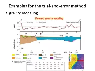
Examples for the trial-and-error method • gravity modeling
Waveform modeling Sidao Ni et al. Science 296, 1850 (2002)
SA exmaple F(x,y) has its global maximum value of 1.0 at x = 0, y = 0. However, it also has several secondary maxima Error function global maximum at (0, 0)
Effect of T on pdf distribution T = 1 T = 10 T = 0.1 T = 0.01 The effect of this temperature T is to exaggerate or accentuate the differences between different values of the error function.
Figure 4.5. For a model with 8 model parameters (each having 8 possible values) heat bathalgorithm starts with a randomly chosen model shown by shaded boxes in (a). Each modelparameter is then scanned in turn keeping all others fixed. (b) shows scanning through themodel parameter m 2. Thus m26 is replaced with m23 and we have a new model described byshaded boxes in (c). This process is repeated for each model parameter.
Figure 4.6. Model generation probabilities (left) and their corresponding cumulativeprobabilities (right) at different temperatures. At high temperature, the distribution is nearly flatand every model parameter value is equally likely. At intermediate temperature, peaks start toappear and at low temperature, the probability of occurrence of the best solution becomes veryhigh. A random number is drawn from a uniform distribution and is mapped to the cumulativedistribution (fight) to pick a model.
Application of heat bath SAseismic waveform inversion Tk = T0(0.99)k (k: number of iteration) 100 iterations