Solving Linear Systems of Equations
230 likes | 489 Vues
Solving Linear Systems of Equations. Computational Considerations general solution to a system particular solutions: Square systems Overdetermined systems Underdetermined systems. Computational Considerations.

Solving Linear Systems of Equations
E N D
Presentation Transcript
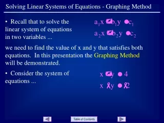
Solving Linear Systems of Equations • Computational Considerations • general solution to a system particular solutions: • Square systems • Overdetermined systems • Underdetermined systems
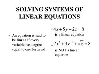
Computational Considerations One of the most important problems in technical computing is the solution of simultaneous linear equations. In matrix notation, this problem can be stated as follows; say by 1-by-1 matrix: 7x = 21 Does it have a unique solution? The answer is yes… x= 3 1-by-1 example.
Computational Considerations • The solution is not ordinarily obtained by computing the inverse of 7, that is 7-1 = 0.142857..., and then multiplying 7-1 by 21. This would be more work and, if 7-1 is represented to a finite number of digits, less accurate. Similar considerations apply to sets of linear equations with more than one unknown;
Computational Considerations • MATLAB uses the division terminology familiar in the scalar case to describe the solution of a general system of simultaneous equations; i.e.; • X = A\B denotes the solution to the matrix Equation AX = B • X = B/A denotes the solution to the matrix equation XA = B You can think of "dividing" both sides of the equation AX = B or XA = B by A. The coefficient matrix A is always in the "denominator
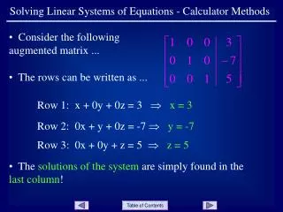
Computational Considerations • The dimension compatibility conditions for X = A\B require the two matrices A and B to have the same number of rows. The solution X then has the same number of columns as B and its row dimension is equal to the column dimension of A. For X = B/A, the roles of rows and columns are interchanged.
Computational Considerations • In practice, linear equations of the form AX = B occur more frequently than those of the form XA = B. Consequently, backslash is used far more frequently than slash.
Computational Considerations • The coefficient matrix A need not be square. If A is m-by-n, there are three cases. • m = n Square system. Seek an exact solution. • m > n Over determined system. Find a least squares solution. • m < n Underdetermined system. Find a basic solution with at most m nonzero components.
Computational Considerations The backslash operator employs different algorithms to handle different kinds of coefficient matrices. The various cases, which are diagnosed automatically by examining the coefficient matrix, include: • Permutations of triangular matrices • Symmetric, positive definite matrices • Square, nonsingular matrices • Rectangular, over determined systems Rectangular, underdetermined systems
General Solution The general solution to a system of linear equations AX = b describes all possible solutions. You can find the general solution by: • Solving the corresponding homogeneous system AX = 0. Do this using the null command, by typing null(A). This returns a basis for the solution space to AX = 0. Any solution is a linear combination of basis vectors. • Finding a particular solution to the non-homogeneous system AX = b. You can then write any solution to AX = b as the sum of the particular solution to AX = b, from step 2, plus a linear combination of the basis vectors from step 1.
Square Systems The most common situation involves a square coefficient matrix A and a single right-hand side column vector b. Nonsingular Coefficient Matrix: If the matrix A is nonsingular, the solution, x = A\b, is then the same size as b. For example,
Example MatLab A = pascal(3); u = [3; 1; 4]; x = A\u • x = • 10 • -12 • 5 It can be confirmed that A*x is exactly equal to u.
Square Matrix If A and B are square and the same size, then X = A\B is also that size. B = magic(3); X = A\B X = • 19 -3 -1 • -17 4 13 • 6 0 -6 It can be confirmed that A*X is exactly equal to B.
Coefficient Matrix • Both of these examples have exact, integer solutions. This is because the coefficient matrix was chosen to be pascal(3), which has a determinant equal to one. A later section considers the effects of roundoff error inherent in more realistic computations.
Singular Coefficient Matrix • A square matrix A is singular if it does not have linearly independent columns. If A is singular, the solution to AX = B either does not exist, or is not unique. The backslash operator, A\B, issues a warning if A is nearly singular and raises an error condition if it detects exact singularity.
Example Singular Coefficient P = pinv(A)*b P is a pseudoinverse of A. If AX = b does not have an exact solution, pinv(A) returns a least- squares solution. For example, A = [ 1 3 7 -1 4 4 1 10 18 ] is singular, as you can verify by typing • det(A) • ans = • 0
Exact Solutions. For b =[5;2;12], the equation AX = b has an exact solution, given by: pinv(A)*b • ans = • 0.3850 • -0.1103 • 0.7066 You can verify that pinv(A)*b is an exact solution by typing A*pinv(A)*b
Verification Example b =[5;2;12]; A = [ 1 3 7;-1 4 4; 1 10 18]; >> A*pinv(A)*b • ans = • 5.0000 • 2.0000 • 12.0000
Least Squares Solutions. On the other hand, if b = [3;6;0], then AX = b does not have an exact solution. In this case, pinv(A)*b returns a least squares solution. If you type:
Least Square Solution b = [3;6;0]; >> A*pinv(A)*b • ans = • -1.0000 • 4.0000 • 2.0000 you do not get back the original vector b.
Has it got exact solution? You can determine whether AX = b has an exact solution by finding the row reduced echelon form of the augmented matrix [A b]. To do so for this example, enter: > rref([A b]) • ans = • 1.0000 0 2.2857 0 • 0 1.0000 1.5714 0 • 0 0 0 1.0000 Since the bottom row contains all zeros except for the last entry, the equation does not have a solution. In this case, pinv(A) returns a least-squares solution.