Chapter 4. Concentrated Solutions and Phase Separation Behavior
Chapter 4. Concentrated Solutions and Phase Separation Behavior. 4.1 Phase Separation and Fractionation. 4.1.1 Motor Oil Viscosity Example.

Chapter 4. Concentrated Solutions and Phase Separation Behavior
E N D
Presentation Transcript
Chapter 4. Concentrated Solutions and Phase Separation Behavior
4.1 Phase Separation and Fractionation 4.1.1 Motor Oil Viscosity Example
The viscosity of today’s motor oils bears designations such a SAE 5W-30. According to crankcase oil viscosity specification SAE J300a, the first number refers to the viscosity at -18 oC, and the second number at 99 oC.
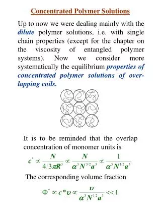
4.1.2 Polymer-Solvent Systems According to thermodynamic principles, the condition for equilibrium between two phases requires that the partial molar free energy of each component be equal in each phase. This condition requires that the first and second derivatives of △G1 with respect to ν2 be zero. The critical concentration at which phase separation occurs may be written For large n, the right-hand side of Eq (4.1) reduces to 1/n0.5.
The critical value of the Flory-Huggis polymer-solvent interaction parameter, c1, is given by which suggests further that as n approaches infinity, c1c approaches 1/2 The critical temperature is the highest temperature of phase separation. The equation for the critical temperature is given by Ψ1is constant
Plot 1/Tc versus 1/n0.5 + 1/2n should yield the Q-temperature at n = infinity fractionation
The Q-temperature for PS/cyclohexane was 34.5 oC. The phase separation curve called binodal line.
4.1.3 Vitrification Effects The effect of the solvent at high polymer volume fraction is to plasticize the polymer. However, if the polymer is below its glass transition temperature, the concentrated polymer solution may vitrify, or become glassy. The vitrification line generally curves down to lower temperatures from pure polymer as it becomes more highly plasticized. Concentration vs. solubility?
The interception of these two curves is known as Berghmans’ point (BP) and defined as the point where the liquid-liquid phase separation binodal line is intercepted by the vitrification curve.
4.2 Regions of the Polymer-Solvent Phase Diagram • A polymer dissolves in two stages: • solvent molecules diffuse into the polymers, swelling it to a gel state. • Then the gel gradually disintegrates, the molecules diffusing into the solvent-rich regions. • In this discussion, linear amorphous polymers are assumed.
φvs.u (excluded volume parameter) Daoud and Jannink and others divided polymer-solvent space into several regions, plotting the volume fraction of polymer, φvs.u (excluded volume parameter) x : screening length dilute solution regime, x = Rg. Semidilute regime, z measures the distance between chain contacts. Cross-linked, x provides a measure of the net size.
The screening length, x, first introduced by Edwards. This quantity takes slightly different meanings in different regimes In the dilute solution regime, x = Rg. In the semidilute regime, x measures the distance between chain contacts. If the polymer is crosslinked, x provides a measure of the net size. For semidilute solutions, the dependence of x onφfollows the scaling lawxs ~ φ-3/4
For semidilute solutions, the dependence of x on j follows the scaling law Another quantity of interest in semidilute solutions is called the blob. It contains a number of mers on the same chain defined by the mesh volume xs3, inside of which excluded volume effects are operative. Some texts define the blob as the number of mers between adjacent entanglements, distance xs apart. These blobs are large enough to be self-similar to the whole polymer chain coiling characteristics; they are coil within coil.
4.3 Polymer-Polymer Phase Separation When two polymers are mixed, the most frequent result is a system that exhibits almost total phase separation. Qualitatively, this can be explained in terms of the reduced combinatorial entropy of mixing. LCST UCST
4.3.1 Phase Diagram Phase separation and dissolution are controlled by three variables: temperature, pressure, and concentration. Lower critical solution temperature (LCST)
Ex: HIPS & ABS Solid line : binodal curve Dash line : spinodal curve
4.3.2 Thermodynamics of Phase Separation The basic equation for mixing of blends reads V : the volume of the sample Vr : the volume of one cell z : the lattice coordination number Nc : the number of cells in 1 cm3 The first term on the right being the heat of mixing term △HM. The second term on the right is the statistical entropy of mixing term, △SM.
4.3.3 An Example Calculation: Molecular Weight Miscibility Limit
4.3.4 Equation of State Theories At equilibrium, an equation of state is a constitutive equation that relates the thermodynamic variable of pressure, volume, and temperature. Imagine that a multicomponent mixture is mixed with No holes of volume fraction υo. Then the entropy of mixing is Noting that the fractional free volume is given by 1-r, the entropy of mixing vacant sites with the molecules in equation of state terminology is given by Where r is less than unity. When all the sites are occupied, r = 1, and the right hand side is zero.
The Gibbs free energy of mixing is given by Where the quantity e* is a van der Waals type of energy of interaction. Note that r = r(P,T); r 1 as T 0; r 1 as P ∞ By taking △Gm/r = 0, the equation of state via the lattice fluid theory is obtain Where r is the number of sites in the chains, and
For high polymers, r goes substantially to infinity, yielding a general equation of state for both homopolymers and miscible polymer blends, The corresponding equation of state derived by Flory is Workers in the field prefer to state the equations in terms of density relations, because for condensed systems, density is easier to measure than volume. Again, r = r/r* = V*/V
This information may be used to determine miscibility criteria The quantity T* and P* represent theoretical values at close packing.
4.3.5 Kinetics of Phase Separation Nucleation and growth Spinodal decomposition
4.3.6 Miscibility in Statistical Copolymer Blends As stated previously, most homopolymer blends are immiscible due to the negative entropy of mixing and negative heats of mixing. Sometimes, however, miscibility can be achieved with the introduction of comonomers.
Karasz and MacKnight approached the problem through mean field thermodynamic considerations, arguing that negative net interactions are necessary to induce miscibility. Where n1 and n2 are volume fractions, n1 and n2 are degrees of polymerization, and cblend is a dimensionless interaction parameter defined as Where the coefficient cij are functions of the copolymer compositions, with 0 ≦ cij ≦ 1. For An/(BxC1-x)n’ blends,
4.3.7 Polymer Blend Characterization Very small size (20 nm) serve to make good damping compositions, while domains of the order of 100 nm make better impact-resistant materials.
Block Copolymer (microphase separation) volume fraction < 0.20 0.20 ~ 0.35 > 0.35
order disorder
Block Copolymer phase diagram disorder
Representative phase diagram of diblock copolymers(Khandpur et al., Macromolecules1995, 28, 8796)
4.3.9 Block Copolymers K is the experimental constant relating the unperturbed root-mean-square end-to-end distance to the molecular weight.
Idealized triblock copolymer thermoplastic elastomer morphology
4.3.11 Ionomers Ionomers are polymers that contain 5% to 15% ionic groups. While these materials are statistical copolymers, the ionic groups usually phase separate from their hydrocarbon-like surroundings thus providing properties resembling multiblock copolymers.
4.4 Diffusion and Permeability in Polymers Permeation is the rate at which a gas or vapor passes through a polymer. The mechanism by which permeation takes place involves three steps: • Absorption of the permeating species into the polymer • diffusion of the permeating species through the polymer, traveling, on average, along the concentration gradient • desorption of the permeating species from the polymer surface and evaporation or removal by other mechanisms. Factors affecting permeability include the solubility and diffusivity of the penetrant into the polymer, polymer packing and side-group complexity, polarity, crystallinity, orientation, fillers, humidity, and plasticization.
4.4.1 Swelling Phenomena If the polymer is glassy, the solvent lowers the Tg by a plasticizing action. Polymer molecular motion increases. Diffusion rates above Tg are far higher than below Tg.